Human Capital Pays, If You Count the Cost: School Funding, State Growth, and a Diverging America

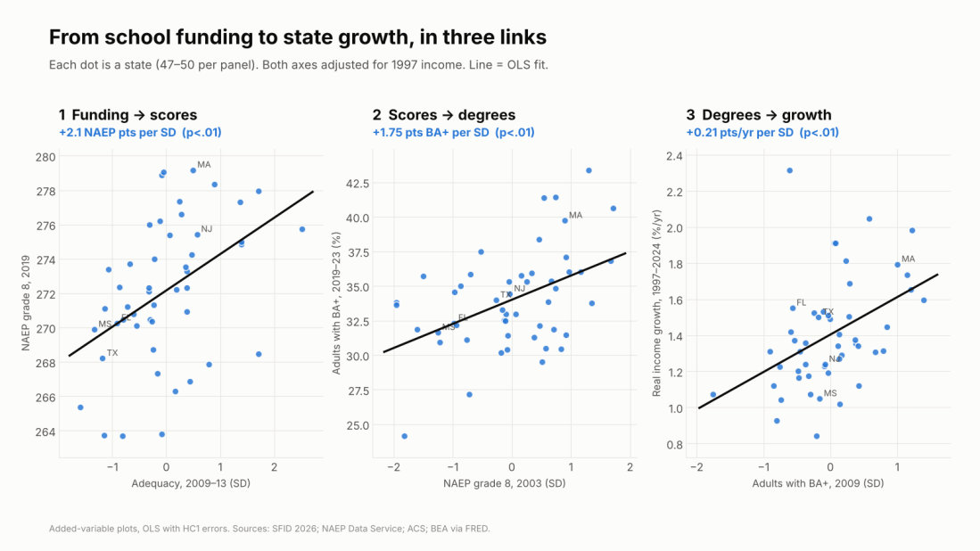
Three scatterplots of states with rising fitted lines: adequacy 2009-13 against 2019 grade 8 NAEP (+2.1 points per SD); 2003 grade 8 NAEP against the share of adults with a BA (+1.75 points per SD); BA share in 2009 against real income growth 1997-2024 (+0.21 points a year per SD). All adjusted for 1997 income.

Economists around the world treat schooling as an investment in human capital: the skills and knowledge that make people, and economies, productive. The international evidence that this investment pays is about as settled as anything in the field. Yet here in the U.S., we keep having the same argument about whether school money matters.

Here’s what I find across the 50 states. Count the school dollar the usual way, adjusted only for teacher wages, and it tells you nothing useful about economic growth since the 1990s. If anything, it points the wrong way. Count it against what it actually costs to build skills, given the kids a state serves, and the human capital chain appears: adequate funding goes with higher 8th-grade scores, higher scores with more college-educated adults, and more college-educated adults with faster income and GDP growth.

The numbers, per standard deviation across states, holding 1997 income constant:

  • Funding → skills: about +2 NAEP points in 8th grade (2019), +1.2 for low-income students, and a 1.5-point smaller gap between them and their peers.
  • Skills → degrees: +1.75 points more adults with a BA in states that scored higher in 2003.
  • Degrees → growth: +0.21 points a year faster real income growth and +0.43 points a year faster GDP per capita growth over 1997–2024.

Put the wage-adjusted dollar and the cost-adjusted dollar in the same model and they split: adequacy predicts +0.39 points a year faster income growth, wage-adjusted spending −0.31. Same states, same years, opposite answers. The difference is whether you counted cost.

Full policy paper (PDF, 24 pages), with complete data sources, variable definitions, model specifications and results: Investing in Human Capital: Does Long-Run K-12 Investment Fuel State Economic Growth?

Schools are a human capital investment, and the world knows it pays

Years of school pay. Harry Patrinos and George Psacharopoulos have spent decades compiling returns to schooling. Their 2018 review pulls together 1,120 estimates from 139 countries and finds an average private return of about 9% per year of schooling (Psacharopoulos & Patrinos, 2018). Their 2025 follow-up looks only at causal estimates, 182 of them from 55 countries, and the return goes up, to 9.7%, about 38% higher than the correlational estimates (Patrinos & Psacharopoulos, 2025).

Learning pays more. One standard deviation higher test scores raises earnings about 15%, roughly one and a half times the value of an extra year of school (Patrinos & Psacharopoulos, 2025). Among adults in 23 countries, a standard deviation of numeracy is worth 18% in wages, and the U.S. pays the most for skills, at 28% (Hanushek et al., 2015). With harmonized learning data for 164 countries, human capital explains one-fifth to one-half of income differences across countries (Angrist, Djankov, Goldberg & Patrinos, 2021).

Skills drive growth. Across countries, a standard deviation higher achievement goes with 1.3 to nearly 2 points faster annual growth over decades (Hanushek & Woessmann; Heller-Sahlgren & Jordahl, 2021). Across U.S. states, knowledge capital explains 20–30% of differences in GDP per capita (Hanushek, Ruhose & Woessmann, 2017).

And it can be lost. Pandemic closures cost students about 0.17 of a standard deviation, half a year of learning (Patrinos, Vegas & Carter-Rau, 2022). The World Bank’s new Human Capital Index Plus puts the U.S. at 252 out of 325, below the high-income average and well behind Australia’s 270 (World Bank, 2026).

Here’s the gap. This literature measures human capital outputs with great care. Its school inputs are usually just spending per pupil, adjusted at most for prices. If schooling is an investment, the right question is whether a state spends enough to produce a given level of skills with the students it actually has. That is a cost question.

Four ways to count a school dollar

There are four common ways to count a school dollar, each correcting for more than the last: nominal; inflation-adjusted; labor-cost-adjusted, using a wage index like NCES’s CWIFT; and fully cost-adjusted, comparing spending with what it would cost to reach a common outcome goal given wages, scale and, above all, student needs. Only the fourth asks whether the money is enough for the job. That is what the School Finance Indicators Database’s National Education Cost Model measures. I’ve made this case in Why “Cost” Matters and Efficiently Mediocre.

Brookings’s state-level report (Reber & Goodman, 2025) stops at number three. Student need goes in as a control variable, not as a cost. That treats a dollar spent on a high-poverty student body as worth the same as a dollar spent on a low-poverty one, then controls away the very poverty that makes those dollars unequal. (See Mark Weber’s NEPC review.)
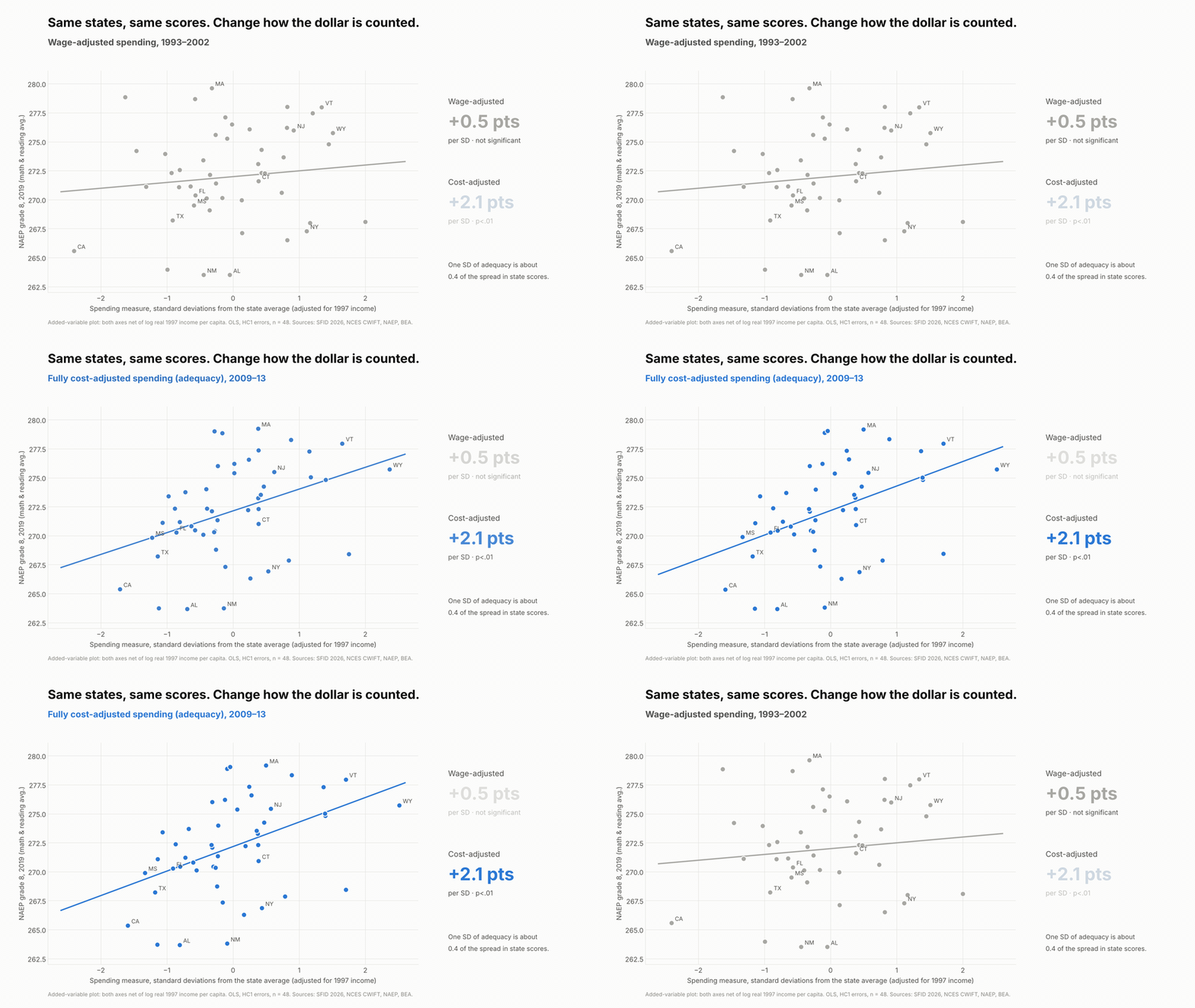
Animated scatterplot of 48 states: against 2019 grade 8 NAEP, wage-adjusted spending shows a flat line (+0.5 points per SD, not significant); measured against the cost of U.S.-average outcomes, the line steepens to +2.1 points per SD.
Same states, same scores. Change how the dollar is counted. Both axes adjusted for 1997 income.

The human capital chain: investment → skills → degrees → growth

The setup is simple. Take state economic outcomes over 1997–2024 from BEA, and compare them with K-12 conditions earlier in the period: wage-adjusted spending from 1993–2002, NECM adequacy from 2009–13, NAEP from 2003, and adult BA attainment. Control for each state’s real income in 1997 so rich states don’t win just for starting rich. Everything is per standard deviation across states, with robust standard errors.

Link 1: investment → skills. A standard deviation of adequacy goes with about 2.1 NAEP points on the 2019 state average, +1.2 for low-income students, and a 1.5-point smaller gap. Wage-adjusted spending: +0.5, not significant. The adequacy link holds with the Northeast dropped (+2.2).

Link 2: skills → degrees. States whose 8th graders scored a standard deviation higher in 2003 have 1.75 points more adults with a BA today, and they added about half a point more BA holders between 2009 and 2024 as those kids grew up.

Link 3: human capital → growth. A standard deviation more BA holders in 2009 goes with 0.21 points a year faster real income growth and 0.43 points faster GDP per capita growth. Higher 2003 NAEP goes with +0.12 and +0.23. Low-income students’ scores predict growth just as well (+0.14 and +0.21), and those estimates survive dropping the energy and resource states.
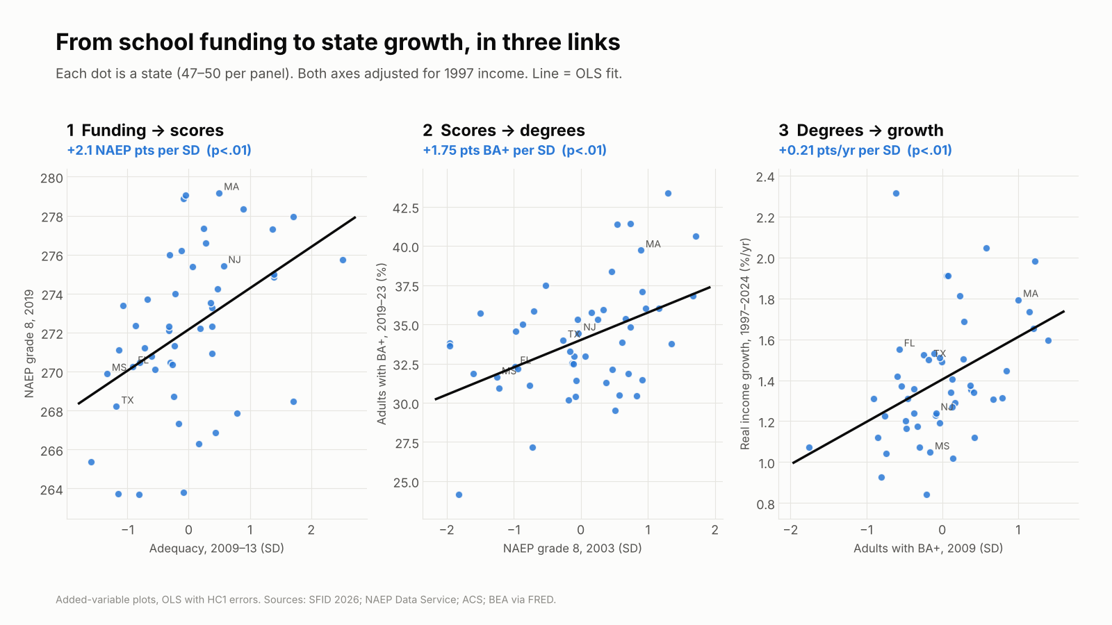
Three scatterplots of states with rising fitted lines: adequacy against 2019 NAEP (+2.1 points per SD); 2003 NAEP against BA attainment (+1.75 points per SD); BA share in 2009 against real income growth 1997-2024 (+0.21 points a year per SD).
Each dot is a state. Both axes adjusted for 1997 income; lines are OLS fits.

How the state numbers stack up against the world

States differ far less than students do. A standard deviation across states on 2003 NAEP is 6.5 points, about a sixth (0.17) of a student-level standard deviation. Scale the international estimates by that and the state results land right where you’d expect:

Global benchmark, per student SDImplied for 1 state SDWhat I find
Skills → GDP per capita growth+1.3 to +1.86 pts/yr+0.22 to +0.31 pts/yr+0.23 pts/yr
Skills → earnings+15% (Patrinos & Psacharopoulos); +28% in the U.S. (Hanushek et al.)+2.5% to +4.6%About +3.3% higher real income after 27 years
Dollars → skills+0.032 SD per $1,000 for four years (Jackson & Mackevicius, 2024)—About +0.012 SD per $1,000 of adequacy

The growth estimate sits inside the range the cross-country studies predict; +0.23 points a year compounds to a GDP per capita level about 6% higher over 27 years. The funding estimate, per dollar, is about a third of the causal estimate from U.S. school finance evaluations: modest, not inflated. These are rough conversions across different tests, but nothing here is out of line with what the human capital literature would lead you to expect.

Diverging states, diverging futures

Here’s where I want to be blunt. The United States does not have one human capital system. It has fifty, and they are sorting into leaders and laggards.

  • Attainment is diverging. States with more college graduates in 2009 added more of them by 2024. The five most-educated states went from 36% to 46% of adults with a BA; the five least-educated went from 20% to 27%. The gap widened from 16 to 19 points.
  • The economic extremes are pulling apart. Massachusetts’s GDP per capita was 1.6 times Mississippi’s in 1997 and 2.2 times in 2024. For most of the twentieth century, poorer states caught up with richer ones; Ganong and Shoag show that convergence has slowed dramatically over the past three decades.
  • The skills gap between states is an international-scale gap. In the most recent state-by-country comparison, the 2011 NAEP–TIMSS linking study, Massachusetts’s 8th graders scored 561 in math, behind only five of 47 education systems, the closest being Japan. Alabama scored 466, statistically tied with Turkey and Armenia. That 95-point spread is close to a full international standard deviation, a gap that across countries goes with 1.3 to 1.9 points of annual growth.
  • The funding gaps behind it are persistent. States’ adequacy positions barely move over a decade (correlation 0.92). Mississippi spent about half of what its students needed in 2009–13 and was still $9,300 per pupil short in 2021–23, and $25,100 short in its highest-poverty districts.
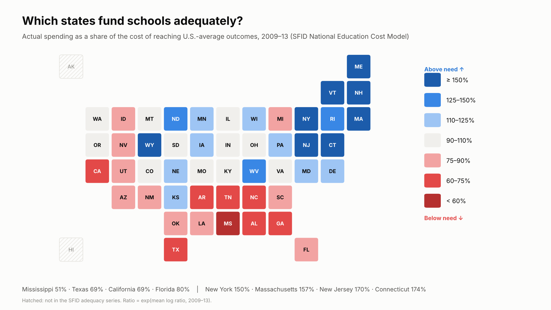
Tile-grid map of states colored by spending as a share of the cost of reaching U.S.-average outcomes, 2009-13. The Northeast is dark blue (Connecticut 174%, New Jersey 170%, Massachusetts 157%, New York 150%); the South is mostly red (Mississippi 51%, Texas and California 69%, Florida 80%).
Actual spending as a share of the cost of reaching U.S.-average outcomes, 2009–13 (SFID National Education Cost Model).

The knowledge economy concentrates where human capital is. Research universities, technology industries and scientific talent cluster in states with deep pools of skilled workers, and those states draw more of them. If current funding patterns hold, the leading states will keep compounding that advantage. The lagging states will keep producing fewer skilled workers, attracting fewer knowledge industries, and losing many of the graduates they do produce.

Let me be precise about how far this goes. No state is about to become a developing country in income. Mississippi’s GDP per capita, $41,300 in 2024, is far above most of the world’s, propped up by a national labor market and federal transfers. But on skills, our lowest-performing states already score alongside upper-middle-income countries such as Turkey and Armenia, while our highest-performing states compete with Japan. Skills set the ceiling on what an economy can become. A country that draws its scientists, engineers and entrepreneurs from a handful of states is leaving most of its human capital on the table. Because states and localities supply most K-12 funding, the path forward for American economic and scientific development runs through state investment in human capital, measured against what it actually costs to build it.

A note on California. California sits near the bottom of the map above, which shows 2009–13, and it still falls short of adequate funding today, especially in its highest-poverty districts. But in my analyses, no state has improved more since 2009. As I showed in The Red State Miracle That Wasn’t, California’s highest-poverty districts went from 65% to 79% of adequate funding between 2009 and 2024, most of it after the Local Control Funding Formula began phasing in after 2013, though they remain about $5,600 per pupil short. In the state data behind this post, California climbed from 45th of 48 states on adequacy in 2009–13 to the middle of the pack by 2021–23. California is digging out of a very deep hole. The 1978 tax revolt, Proposition 13, capped property taxes at 1% of assessed value and gutted the local revenue that had supplied about two-thirds of school funding.

What this does and doesn’t show

These are cross-state associations, not causal estimates. College graduates move, so a state’s BA share partly reflects whom it attracts. Adequacy is measured in 2009–13, inside the growth window, so faster-growing states may simply have afforded better-funded schools. And required cost reflects student need, which also lowers scores. The paper documents each of these and the robustness checks behind them.

But the stronger designs point the same way. Jackson and Mackevicius (2024) pool U.S. school finance evaluations and find that $1,000 more per pupil for four years raises test scores by 0.032 SD and college-going by 2.8 points. Jackson, Johnson and Persico find that sustained spending increases raise adult wages. And the international lesson from Patrinos and Psacharopoulos is that causal returns to education run higher than correlational ones. If anything, cross-state associations like mine are more likely to understate the human capital return than to invent it.

The bottom line

Around the world, nobody serious doubts that human capital pays. A year of school is worth about 9–10% in earnings, a standard deviation of learning about 15%, and a country’s skills go a long way toward explaining its growth. The U.S. debate gets stuck because it measures the investment badly. Measure it against the cost of building skills, and the return shows up across the states just as it does across countries: funding to skills, skills to degrees, degrees to growth.

The states are not converging; at the top and bottom they are pulling apart. Whether America remains an economic and scientific leader depends on whether every state invests in the human capital of all its children, and especially the children who rely most on public schools, or whether we settle for a few states that lead and many that fall further behind.

Read the full policy paper (PDF): Investing in Human Capital: Does Long-Run K-12 Investment Fuel State Economic Growth? It includes all data sources, variable definitions, model specifications, robustness checks, a full table of results and replication details.

Data: BEA via FRED; School Finance Indicators Database (2026); NCES ACS-CWIFT; NAEP Data Service; ACS. International sources are listed in the paper.
Transcript of Video Critiquing Edunomics Graphs

“Make it stop! Please!” — Video debunking of Edunomics intentionally deceitful school funding/outcome graphs

Source: School Finance 101 (Bruce Baker), published June 16, 2026

schoolfinance101.com — Make it stop! Please!

Transcribed from the post’s auto-generated captions (video runtime ≈ 20 minutes) and lightly cleaned up for readability; screenshots below are frames pulled from the same video at the points the graphs are shown on screen. A few short passages were unintelligible in the source captions and are marked accordingly.

Greetings, folks. Let’s talk. I need to vent a little bit, because after all these years, the same BS continues to roll out, continues to emerge in the school finance conversation — something I’ve been writing and talking about for years.

I put this report out last year, this new version of Does Money Matter in Education? — summarizing a whole bunch of rigorous, peer-reviewed studies applying different approaches and using different data that show us how and why money matters for improving student outcomes.

I talked about this years ago — for a decade, really. This is actually a little less than a decade old, in this book and in other sources on my blog going back more than a decade: basically the dumbest, most facile, simple-minded, intentionally deceitful versions of arguments that try to say, well, money doesn’t really matter. You can do great — you can be awesome with very little money — and you can suck with lots of money. Money’s gone up and test scores have gone down. There are really about four or five different versions of this argument that have been thrown out over the years, but there are two common ones — pretending to be empirical analyses — that are repeatedly used, and that I’ve repeatedly debunked, that just continue to find their way back.

At this point, anyone who’s putting these kinds of graphs out there is doing so knowingly and intentionally to deceive policymakers, courts, judges — whatever. Most of this stuff doesn’t make its way these days into judicial debates over school funding, but I had to face this again over a year ago, and then I’ve seen these graphs re-emerging for every state continuously over the past year — and even again recently on Twitter/Bluesky, where one of my colleagues, thankfully, also took a shot at just how stupid and intentionally deceitful these graphs are.

So let’s jump into it. If you’re a policymaker in a state — or if you know one, or if you’re on a commission in a state and people have been invited in and are putting this stuff in front of you — stop it right there. Kick them out of the room. This is not credible. It shouldn’t be part of the discussion. Just look at the graph.

Graph #1: The “long-term trend” graph

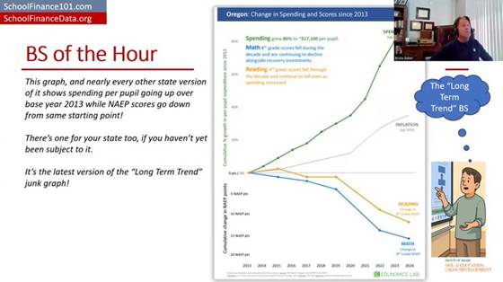
Here’s one of the graphs — this is the new version of what I call the long-term trend graph. The Edunomics Lab at Georgetown University — I’ll call them out by name — and Marguerite Roza have put out data visualization tools that let you make this graph for every state, and then the next graph I’ll talk about.

Let’s take a look at this. First of all — and I’ll explain why this is part of the intentional deceit — they picked 2013 as the starting year. Second, you get two totally different kinds of measures put on a common y-axis, a common vertical axis, with different units for the test scores than for the spending, and both of them stretched out to make it look like these trends are wildly diverging.

Edunomics-style “long-term trend” graph for Oregon: spending, NAEP math/reading, and inflation all plotted on a common stretched axis since 2013 (“BS of the Hour” slide).

And even the construction of the measures is a problem. We’ve got per-pupil spending, not even adjusted for inflation, and then a separate line for some inflation adjustment — maybe a Consumer Price Index — which isn’t even the right adjustment to use for per-pupil spending. I’ll show you what it looks like adjusted correctly in a few minutes.

They’ve got per-pupil spending skyrocketing. I’m using Oregon here because it’s the last place I was faced with having to waste an exorbitant amount of time debunking this garbage. So we’ve got per-pupil spending — not adjusted for inflation, just nominal per-pupil spending — seemingly skyrocketing, which you can do by stretching out the y-axis. And we’ve got NAEP (National Assessment of Educational Progress) test scores taking a dive from 2013 forward to 2024. Then there’s a separate, gratuitous inflation measure thrown in on yet another scale. My head explodes just looking at this. And most people who’ve encountered this graph and have any knowledge of how to do actual research and empirical analysis, and how to measure a school dollar — their heads have exploded too.

Why 2013 is the tell

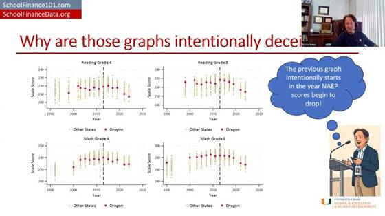
Let’s talk about 2013 for a second. First, 2013 is well understood to be the point at which NAEP scores level off and/or start to decline. They go up for all the years before that, and then they hit a plateau and start to decline. So picking 2013 is intentionally picking the point at which, in almost any state, you can show test scores leveling off or going down while money is going up or staying the same — which, of course, looks bad. It implies money couldn’t possibly relate to test scores. Better research says otherwise, even for this period.

NAEP Grade 4 Reading and Grade 8 Math scores over time for all states, with Oregon highlighted — scores plateau/decline for nearly every state starting around 2013.

Here’s NAEP scores over time for all states, with Oregon highlighted — and, like the others, it just drifts downward from that point, more or less within the pattern of other states (a bit more so for the fourth-grade scores). But picking 2013 was intentionally picking the year at which NAEP scores level off or turn downward.

On the spending side: per-pupil spending for public school districts took a real hit starting around 2008–09. 2008 was about the best year for public school expenditures. From about 2008–09 to about 2011–12 is when spending really took a hit. It had drifted upward through 2008, then dips, and hits its bottom — leveling off and maybe starting to creep back upward a little around 2013.

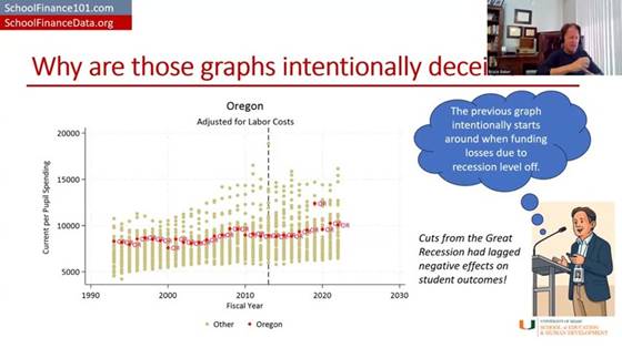
Oregon per-pupil spending by fiscal year, adjusted for labor costs, compared to other states — spending bottoms out around 2013 after the Great Recession before drifting back up.

So if you pick 2013 as your starting point, what you’re actually picking is the year when the cuts to funding had hit bottom and test scores had hit their peak. Track it forward from there for almost any state, and you’ll get this apparent divergence — especially once you consider that spending should really be adjusted for the cost of recruiting and retaining a comparable-quality teacher workforce, given that private-sector and other wages have been rising faster than wages for teachers and public school employees. Adjusted that way, spending clearly does not skyrocket the way it does in their graph. Again, 2013 is right where spending per pupil bottoms out and levels off (maybe starts to climb a little) — stretch the axis and don’t adjust for anything, and you can make it look like it’s climbing a lot.

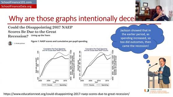
Interesting side note: there’s a really good empirical study by Jackson and coauthors (published via EducationNext) that shows the detrimental effects of recessionary cuts on student outcomes during that exact same period.

“Could the Disappointing 2017 NAEP Scores Be Due to the Great Recession?” (EducationNext) — Figure 1: NAEP scores and cumulative per-pupil spending, zoomed in on 2000–2015.

Zooming in on just the 2000–2015 period the way this study does, test scores actually rose when spending rose, leveled off when spending leveled off, and dipped when spending dipped — the opposite pattern from what’s implied by stretching the axes the way Edunomics does. That study’s authors go on to run solid, causal empirical analyses of this relationship — including, later, a study with more than 30 causal estimates of the returns to a $1,000 increase in public school expenditure, which I summarize along with a ton of other studies in my report.

And yet the graph still persists. It’s still thrown at us in the most absurd ways.

A properly adjusted version

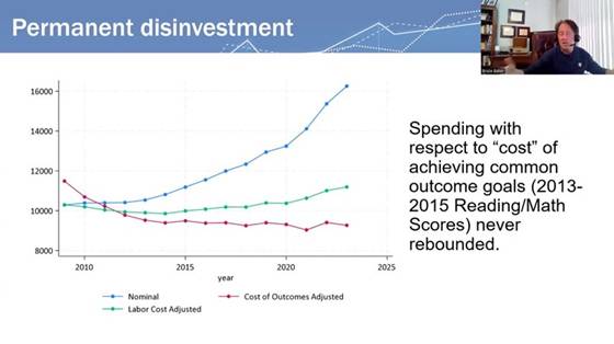
Here’s another version of the graph — the blue line is roughly their version of per-pupil expenditures, though not as exaggerated as showing it as a percent change since 2013 on a stretched y-axis. Just unadjusted per-pupil spending: it went up. Adjusted for changes in labor costs, per-pupil spending is only ever so slightly higher in 2024 than it was in 2009 — that’s adjusting for what it costs to recruit and retain teachers of comparable qualifications.

Now, if we adjust for all of the other cost changes — the student populations to be served, and everything else that goes into achieving a common set of outcomes, using our National Education Cost Model at schoolfinancedata.org — spending actually declined precipitously during and in the years immediately following the fiscal-austerity period after the Great Recession, then levels off, and may even continue drifting down slightly relative to what the dollar was worth toward achieving 2009-level outcomes.

“Permanent disinvestment” — spending with respect to the cost of achieving common outcome goals (nominal vs. labor-cost-adjusted vs. fully cost-of-outcomes-adjusted); the cost-adjusted line never rebounds after the Great Recession.

That’s what fully cost-adjusted spending looks like over time, in many if not most states.

Graph #2: The cross-sectional “spending vs. proficiency” scatterplot

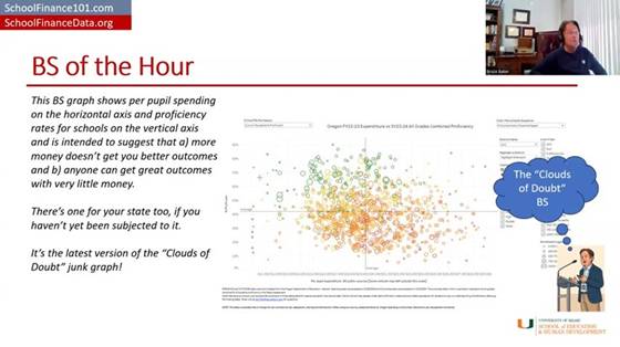
Now for graph number two — another mind-bogglingly, intentionally deceitful graph. The idea: take a whole bunch of schools across a state, regardless of differences in cost from one place to another or the students being served — schools of different grade levels and everything — and plot their per-pupil spending on the horizontal axis and their percent proficiency on state tests on the vertical axis.

The “Clouds of Doubt” graph: Oregon FY22–23 per-pupil expenditure vs. SY23–24 all-grades combined proficiency, with no cost adjustment — no visible relationship between spending and outcomes.

That lets you show that some schools do awesome with very little money, and some schools do crappy with a whole lot of money — so clearly, money doesn’t matter. That low-spending, high-scoring school just needs everyone else to learn from its awesomeness, and everyone can be awesome with whatever they have. Inequity doesn’t matter, adequacy is irrelevant — just get the better outcome, and if you don’t, it’s because you suck.

The layers of problems with this graph are mind-boggling. The main issue is the complete failure to adjust for the value of the school dollar toward achieving these outcomes from one place to the next — to look at the dollar adjusted for its value, or for whether it’s sufficient to achieve a given target given those outcomes.

What it looks like adjusted for cost

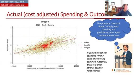
I can give a couple of examples of what happens when you do that adjustment. First, I put Oregon in the context of the nation for 2023. If you look at that unadjusted, the overall pattern looks downward — the more money you have, the worse you do, as if you just don’t know how to use it well, and need to be squeezed harder to perform like the districts in the upper-left corner.

But if instead you responsibly use methods that have been in the peer-reviewed literature going back to about 1971 — and extensively since about 1998–99, in the “modern era” starting with a piece by Downes and Pogue in the early 1990s — and look at each district’s spending relative to what it would cost that district to achieve national-average outcomes, and then look at their actual outcomes relative to the national average, districts that spend more (relative to their cost of achieving average outcomes) achieve more, on average.

“Actual (cost adjusted) Spending & Outcomes” — Oregon districts (red) against the national distribution (gray): funding gap to the cost of national mean outcomes vs. outcome index. A clear, strong, positive relationship.

Districts on the right-hand side of this picture are ones spending more than they’d need to achieve national-average outcomes, and the districts in the upper-right quadrant are mostly achieving above-average outcomes. Districts in the lower left have less funding than needed to achieve national-average outcomes — and guess what, they’re achieving below-average outcomes.

There’s still variation around that trend line — more adequate funding (controlling for costs) generally means better outcomes, but there’s variation worth exploring further, which my colleagues and I have done in individual states. For example, a report on Colorado compares districts and schools that get better outcomes than would be expected given their spending. Sometimes what we find is that there was simply something our model didn’t fully capture about that school or district; sometimes we get real insight into what they’re doing differently. That’s what real efficiency analysis looks like — not making a judgment with no consideration at all for the value of the school dollar.

This other stuff — the raw scatterplot — is garbage. Just say it bluntly: it’s garbage. It’s intentionally deceitful. It has no place in a real policy conversation about how to help schools improve, or how to equitably and adequately fund schools. It shouldn’t be part of the conversation, and neither should the long-term trend graph. It’s utterly ridiculous.

A side-by-side, nationwide comparison

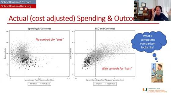
Here’s a side-by-side comparison. If I take districts across the whole country and just look at their per-pupil spending relative to the average for their labor market (i.e., adjusted for regional cost differences in the labor market — from Kansas City to El Paso to New York) — districts spending more than their labor-market average versus less — and plot that against an outcome index combining reading and math scores for grades three through eight, it looks a lot like the Edunomics-style graph: overall, the higher-spending districts don’t appear to be doing any better.

“What a competent comparison looks like” — left: spending/labor-market mean vs. outcomes with no cost control; right: current spending as % of adequate spending (cost) vs. outcomes, with cost control. The relationship only emerges once cost is controlled for.

But if you instead adjust properly for the full cost of achieving a given outcome goal and then plot it, districts with more adequate spending relative to that cost have higher outcomes, and districts with less adequate spending have lower outcomes. Then you can start to explore what explains the variation among districts at similar levels of spending and outcomes — but you can’t make any judgment at all from the unadjusted version. Putting that unadjusted version in front of policymakers or any audience — or, for that matter, using it to teach and train people in a school finance certificate program — is reckless, irresponsible, and needs to stop.

Oregon, school level

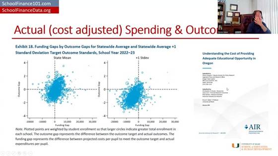
Here’s what it looks like in Oregon with school-level data, based on a report I produced with colleagues at the American Institutes for Research.

AIR’s “Understanding the Cost of Providing Adequate Educational Opportunity in Oregon” (Feb. 2025) — Exhibit 18: funding gaps by outcome gaps for statewide-average and +1 SD target outcome standards, school year 2022–23.

It’s a messy graph, but it generally trends upward, and the statistical analyses in the report show that schools with more adequate funding tend to have higher outcomes, and schools with less adequate funding tend to have lower outcomes. And when you set a higher outcome goal, it costs more to reach it. That’s the punchline.

Closing

This isn’t new, and it shouldn’t come as a surprise to anyone. I called graphs like the second one “clouds of doubt” in my 2018 book — clouds of doubt and the long-term trend were two of the most deceitful ways people tried to argue that schools just need to do better with what they’ve got, that more money doesn’t matter, that we should stop “throwing money” at schools because outcomes are declining anyway. All of that is garbage, and it’s well understood to be garbage. These particular empirical representations of it are an absolute joke.

Stop it now. Shut the door on it. Kick it out of the room. It has no place here, period.

Thank you, and have a wonderful day — I’ve enjoyed this pleasant time chatting with you.

Referenced reports

Baker, Bruce D. (2025). Does Money Matter in Education? (Third Edition). Albert Shanker Institute. shankerinstitute.org/resource/does-money-matter-in-education — PDF: moneymatters3rdedition_final.pdf

Baker, Bruce D., & Losen, Daniel J. (2026). Unpacking Racial Disparities in School Spending: Why “progressiveness” and “comparability” are not enough. EdWorkingPaper ai26-1558, Annenberg Institute at Brown University. edworkingpapers.com/ai26-1558

Brooks, Christopher D., Levin, Jesse, Salvato, Brad, & Baker, Bruce D. (2025). Understanding the Cost of Providing Adequate Educational Opportunity in Oregon. American Institutes for Research, prepared for the Oregon Legislative Policy and Research Office. air.org PDF