The Center for American Progress released its new Return on Investment (ROI) Index for K-12 public school districts of greater than 250 students this week. I should note in advance that I had the opportunity to provide advice on this project early on, and occasionally thereafter and I do believe that at least some involved had and still have the best intentions in coming up with a useful way to represent the information at hand. I’ll get back to the validity of the information at hand in a moment.
First, I need to point out that the policy implications and proposals, or even general findings presented in the report cannot be supported by the analysis (however well or poorly done). The suggestion that billions of dollars might be saved nationally (little more than a back-of-the-napkin extrapolation) at no loss to performance outcomes, based on the models estimated is a huge, unwarranted stretch and quite simply arrogant, ignorant and irresponsible.
The method used provides no reasonable basis for the claim that all low “rate of return” districts could simply replicate the behaviors of high “rate of return” districts and achieve the same or better outcomes at lower cost. The limitations of these methods, when applied in their best and most rigorous complete possible form, no less in this woefully insufficient and incomplete form simply do not allow for such extrapolation.
Further, given the crudeness of the models and adjustments used in the analysis, it is inappropriate to make too much, if anything of supposed differences in the characteristics of districts with good versus bad rate of return indices. You can do some fun hunting and pecking through the maps, but that’s about it!
For example, one major finding is that districts with good ROI’s spend less on administration. However, much more rigorous studies using better data and more appropriate models exploring precisely the same question have found the opposite. The CAP ROI methods are insufficient to draw any conclusion in this regard.
There is little basis in this analysis that states need to provide fairer funding – except that funding does appear to vary within states. But how funding varies is not explored. I like the idea of improving funding fairness, but a better basis for that argument can be found here: www.schoolfundingfairness.org.
And there is no basis for suggesting that fairer funding would be accomplished by student-based funding. Evidence to the contrary might be found here: http://epaa.asu.edu/ojs/article/view/5. This is report writing 101. Be sure that your policy implications follow logically from your findings, and that your findings are actually justified by your analysis.
It was also concluded that on average, higher poverty districts are simply less efficient. When you estimate a model of this type, where you are trying to account for various factors, such as cost factors, outside the control of local school districts – but you aren’t really sure you’ve accomplished the task – when you see a result like this it is a rather basic step to ask yourself – Did I really control sufficiently for costs related to child poverty? Is this finding real? Or is it an indication of bias in my model? A failure to capture real, important differences in the characteristics of these districts?
That single bias – failure to fully account for poverty related costs – is pervasive throughout the entire CAP ROI analysis. There is a strong relationship between poverty and supposed inefficiency in most states in the analysis. That bias exists in states where the state has provided additional resources to higher poverty districts, making them higher spending on average, and that bias exists even in states where spending per pupil is systematically lower in higher poverty districts. And every map and scatterplot in the analysis must be viewed carefully with an understanding of the pervasive, uncontrolled bias against higher poverty districts. A bias that results largely from failure to fully account for cost variation.
Okay, now that I’ve said that rather bluntly, let’s walk through the three different ROI approaches, and what they are missing.
Basic ROI
In any of the ROI’s you’ve got two sides to the analysis. You’ve got the student outcome measures (which I’ll spend less time on), and you’ve got the per pupil spending measures. Within the per pupil spending measures, you’ve got cost adjustments for the “cost” of meeting student population needs and cost adjustments for addressing regional differences in competitive wages for school personnel. The Basic ROI uses an approach similar to that used by Education Week in Quality Counts as a basis for calculating “cost adjusted spending per pupil.”
Weighted Pupil Count = Enrollment + .4*Free Lunch Count + .4*ELL Count + 1.1*IEP Count
After using the weighted pupil count to generate a student need adjustment, CAP uses the NCES Comparable Wage Index to adjust for regional variation in wages. So, they try to adjust for student needs, using a series of arbitrary weights, and for regional wage variation.
The central problem with this approach is that it relies on setting rather arbitrary weights to account for the cost differences associated with poverty, ELL and special education. And in this case, CAP, like Ed Week, shot low – claiming those low weights to be grounded in research literature, but that claim is a stretch at best and closer to a complete misrepresentation. More below.
Adjusted ROI
For the adjusted ROI, CAP uses a regression equation which compares the actual spending of each district to the predicted spending of each district, given student population characteristics. Here’s their equation:
ln(CWI adjusted ppe)= β0 + β1% free lunch + β2 % ELL+ β3 % Special Ed + ε
Now, this method is a reasonable one for comparing how much districts spend, but has little or nothing to do with adjusting for the costs of achieving comparable educational outcomes – a true definition of cost. That is, one can use a spending regression model to determine if a state, on average spends more on high poverty than on low poverty districts. But this is a spending differential not a cost factor. It’s useful, and has meaning, but not the right meaning for this context. One would need to determine how much more or less needs to be spent in order to achieve comparable outcomes.
So, for example, using this approach it might be determined that within a state, higher poverty districts spend less on average than lower poverty districts. This negative or regressive poverty effect would become the cost adjustment. That is, it would be assumed that higher poverty districts have lower costs than lower poverty ones. NO. They have lower spending, but they still most likely have higher costs of achieving constant educational outcomes. Including outcomes and holding outcomes constant is the key – AND MISSING – step toward using this approach to adjust for costs.
Further, the overly simplistic equation above completely ignores significant factors that do affect cost differences and/or spending differences across districts, such as economies of scale and population sparsity as well as more fine grained differences in teacher wages needed to recruit or retain comparable teachers across districts of differing characteristics within the same labor market.
Predicted Efficiency
Finally, there’s the predicted efficiency regression equation, which attempts to generate a predicted achievement level based on a) cost adjusted per pupil spending, b) free lunch, ELL and special education shares. This one, like the others doesn’t attempt to adjust for economies of scale or sparsity and suffers from numerous potential problems with figuring out how and why each district’s actual performance differs from its predicted performance.
achievement = β0 + β1 ln(CWI adjusted ppe) + β2 % free lunch + β3 % ELL + β4 %Special Ed + ε
In this (dreadfully over-) simplified production function approach, any individual district’s actual outcomes could be much lower than predicted or much higher than predicted for any number of reasons. It would appear from scanning through the findings that this particular indicator is most biased with respect to poverty.
Summary of what’s missing or mis-specified
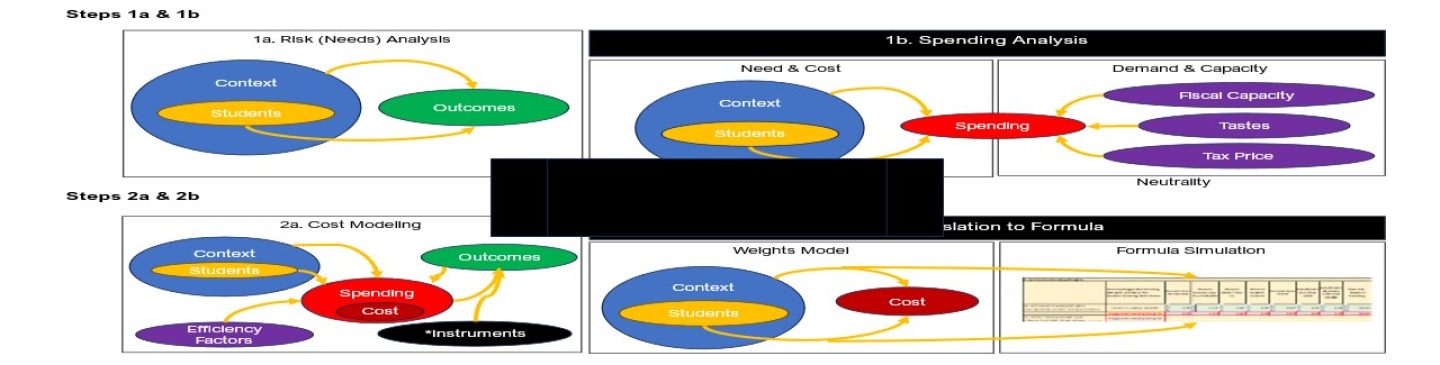
The table below summarizes the three ROI indices – or at least the “adjusted expenditure” side of those indices – with respect to what we know are the major cost factors that must be accounted for in any reasonable analysis of education spending data in relation to student outcomes. Here, the basic conception of cost, and cost difference is “what are the differences in cost toward achieving comparable outcome objectives?” Cost cannot be estimated without an outcome objective.
First, I would argue that the selected weights in the Basic ROI are simply too low, especially in certain parts of the country.
Second, none of the models address economies of scale. CAP notes this, but in a section of the report most will never read. Instead, we’ll all see the pretty maps that tell us that all of the rural districts in the upper Hudson Valley in NY State or in north Central Pennsylvania are really, really inefficient.
Third, recall that the “adjusted ROI” model really doesn’t control for cost at all, but rather for underlying spending variation, without respect for outcomes.
Table 1

Regarding pupil need weights in particular, there exists at least some literature – the most rigorous and direct literature on the question – which suggests the need for much higher weights than those used by CAP. For example, Duncombe and Yinger note that in two versions of their models:
Overall, this poverty weight ranges from 1.22 to 1.67 (x census poverty rate), the LEP weight ranges from 1.01 to 1.42, and the special education weight varies from 2.05 to 2.64.
Across several models produced in this particular paper, one might come to a rounded weight on Census poverty of about 1.5 or weight on subsidized lunch rates of about 1.0 (100% above average cost, or 2x average, more than double the CAP weight), a weight on limited English proficient students around 1.0 and on special education students over 2.0 (slightly less than double the CAP weight).
Other work by me, along with Lori Taylor and Arnold Vedlitz, done for the National Academies of Science, reviewing numerous studies also comes to higher average weights – using credible methods – for children in poverty.
While one can quibble over the selection of “cost” weights from literature, the bigger deal for me remains that the findings of the various ROIs reflect such a strong bias that any reasonable researcher would be obligated to explore further, and perhaps test out alternative research based weights as a way to reduce the bias. It’s a never ending battle, and when you’ve improved the distribution in one state, you’ve likely messed it up in another (because different patterns of poverty and distributions of ELL children lead to different appropriate weights in different settings – even within a state). But this happens – if it turns out to simply be unreasonable to identify a global method for estimating ROIs across school districts and across states, THEN STOP!!!!! DON’T DO IT!!!!! IT JUST DOESN’T WORK!!!!
Here is an example of how much a corrected cost adjustment might matter, when compared with the Basic ROI. The scatterplot below includes one set of dots (red triangles) which represent adjusted operating expenditures of Illinois school districts using the Basic ROI weights. The other set of dots (blue circles) uses a cost index derived from a more thorough statistical model of the costs of achieving statewide average outcomes for Illinois school districts. For the highest poverty districts, the adjusted spending figures drop by $4,000 to $5,000 per pupil when the more thorough cost adjustment method is used. This is substantial, and important, since the ROI is much more likely to identify these districts as inefficient and might be used by state policy makers to argue that cuts to these districts are appropriate (when they clearly are not).
Figure 1

How you specify models to identify efficient or inefficient districts matters, a lot!
Here’s one example of how this type of analysis can produce deceiving results, simply based on the “shape” of the line fit to the scatter of districts. Below is a scatterplot of the cost adjusted spending per pupil for Illinois school districts (unified K-12 districts) in 2008, and the proficiency rates (natural log) for those districts. In this case, I’m actually using much more fully cost adjusted spending levels, accounting for regional and more local wage variation, accounting for desired outcome levels, for poverty, language proficiency, racial composition and economies of scale. As a result, the graph actually shows a reasonable relationship between cost adjusted operating expenditures per pupil and actual outcomes. Spending – when appropriately adjusted – is related to outcomes.
Figure 2

Even then, it’s a bit hard to figure out what shape “best fit” line/curve should go through this scatter. If I throw a straight line in there, and compare each district against the straight line, those districts below the line at the left hand side of the picture are identified as really inefficient – getting much lower outcome than the trendline predicts. But, if I were to fit a curve instead (I’ve simply drawn this one, for illustrative purposes), I might find that some districts previously identified as below the line are now above the line. Are they inefficient, or efficient? Who really knows, in this type of anlaysis!
My biggest problem with the CAP production function analysis is that they came to a result that is so strongly biased on the basis of poverty and instead of questioning whether the model was simply biased – missing important factors related to poverty – they accepted as truth – as a major finding that higher poverty districts are less efficient. It is indeed possible that this is true, but the CAP analysis does not provide any compelling evidence to this effect.
Research literature on this stuff
Note that there is a relatively large literature on this stuff… on whether or not we can, with any degree of precision, classify the relative efficiency of schools or districts. There are believers and there are skeptics, but even among the believers and the skeptics, all are applying much more rigorous methods and refined models and more fully accounting for various cost factors than the present CAP analysis. Here are some worthwhile readings:
Robert Bifulco & William Duncombe (2000) Evaluating School Performance: Are we ready for prime time? In William Fowler (Ed) Developments in School Finance, 1999 – 2000. Washington, DC: National Center for Education Statistics, Office of Educational Research and Improvement.
Robert Bifulco and Stewart Bretschneider (2001) Estimating School Efficiency: A comparison of methods using simulate data. Economics of Education Review 20
Ruggiero, J. (2007) A comparison of DEA and Stochastic Frontier Model using panel data. International Transactions in Operational Research 14 (2007) 259-266
What, if anything, can we learn from those pretty maps and scatters?
Now, moving beyond all of my geeky technical quibbling is there anything we actually can learn from the cool maps and scatters that CAP presents to us. First, and most important, any exploration of the data has to be undertaken with the understanding that all 3 ROI’s suffer from a severe bias toward labeling high poverty urban districts as inefficient and affluent suburban districts as highly efficient (especially in Kansas!). But, with that in mind, one can find some interesting contrasts.
First, I think it would be useful for CAP to reframe and re-label their color schemes. Here’s my perspective on their scatters and color coding. The assumption with the ROI is that there exists an expected relationship between adjusted spending and student outcomes. That’s the diagonal line. Districts in the lower left and upper right are essentially where they are supposed to be. There is nothing particularly inefficient about being in the lower left, or upper right. The use of orange to represent the lower left makes it seem like the lower left is like the lower right. The lower left hand districts in the scatterplot, in theory, are those that got screwed on funding and have low outcomes. Arguably, the lower left hand quadrant of the scatterplots is where one should go looking for school districts wishing to sue their state over inequitable and inadequate funding. These districts aren’t to blame. They are getting what’s expected of them. They are getting slammed on funding and their kids are suffering the consequences – that is, if there really is any precision (which is a really, really suspect assumption) to these models.
Figure 3

Historically, Pennsylvania has operated one of the least equitable, most regressive state school finance formulas in the nation (www.schoolfundingfairness.org). Philadelphia has been one of the least well funded large poor urban core districts in the nation. Strangely, Pittsburgh has made out much better financially. Here’s what happens when we identify the locations of a few Pennsylvania school districts in the CAP ROI interactive tool. I’ve recreated the locations of 4 districts. The location of Philadelphia actually makes some sense on the basic ROI. Philly is royally screwed. Low funding and low outcomes. The implication of the orange shading seems problematic. But if we ponder the meaning of the lower left quadrant it all makes sense. Now, I’m not sure Pittsburgh is really overfunded and/or inefficient, as implied by being in the lower right quadrant – but at least relative to Philadelphia, it does make sense that Pittsburgh falls to the right of Philadelphia on the scatterplot. Lower Merion, an affluent high spending suburb of Philly seems to be in the right place too. I’m not sure, however, what to make of any of the districts, including affluent suburban Central Bucks, which fall in the upper left – the Superstars.
Figure 4
 Because the various ROIs generally under-compensate for poverty related costs, if a district falls in that lower left hand quadrant, we can be pretty sure that the district is relatively underfunded as well as low performing. That is, the district shows up as underfunded even when we don’t fully adjust for costs. This is especially true for those districts that fall furthest into the lower left hand corner. The basic ROI is most useful in this regard, because you know what you’re getting (specific underlying weights). I’ve opened up the comments section so you all can help me identify those notable lower left quadrant districts!
Finally
This type of analysis is an impossible task, especially across all states and dealing with vastly different student outcome data as well as widely varied cost structures. Only precise state by state analysis can yield more useful information of this type. A really important lesson one has to learn when working with data of this type is to realize when the original idea just doesn’t work. I’ve been there a lot myself, even trying this very activity on more than one occasion. There comes a point where you have to drop it and move on. Sometimes you just can’t make it do what you want it to. And sometimes what you want it to do is wrong to begin with. Releasing bad information can be very damaging, especially information of this type in the current political context.
But even more disconcerting, releasing bad data, acknowledging many of the relevant caveats, but then drawing bold and unsubstantiated conclusions that fuel the fire… that endorse slashing funds to high need districts and the children they serve – on a deeply flawed and biased empirical basis – is downright irresponsible.
References
Andrews, M., Duncombe, W., Yinger, J. (2002). Revisiting economies of size in American education: Are we any closer to consensus? Economics of Education Review, 21, 245-262.
Baker, B.D. (2005) The Emerging Shape of Educational Adequacy: From Theoretical Assumptions to Empirical Evidence. Journal of Education Finance 30 (3) 277-305
Baker, B.D., Taylor, L.L., Vedlitz, A. (2008) Adequacy Estimates and the Implications of Common Standards for the Cost of Instruction. National Research Council.
Duncombe, W. and Yinger, J.M. (2008) Measurement of Cost Differentials In H.F. Ladd & E. Fiske (eds) pp. 203-221. Handbook of Research in Education Finance and Policy. New York: Routledge.
Duncombe, W., Yinger, J. (2005) How Much more Does a Disadvantaged Student Cost? Economics of Education Review 24 (5) 513-532
Taylor, L. L., Glander, M. (2006). Documentation for the NCES Comparable Wage Index Data File (EFSC 2006-865). U.S. Department of Education. Washington, DC: National Center for Education Statistics.
 What we see here is that resources – after adjustment for needs and costs – vary widely. Heck, they vary quite substantially even without these adjustments! What we also see is that we’ve got some really high flyers, like Weston, New Canaan and Westport, and we’ve got some that, well, are a bit behind in both equitable resources and outcomes (Bridgeport and New Britain in particular). To be blunt, THIS MATTERS! Yeah.. okay, reformy pundits are saying, but they really have enough anyway. Why put anything else into those rat-holes.


 In this case, imagine trying to recruit and retain teachers of comparable quality in JS Morton to those in New Trier at $20k less on average, or in Aurora East compared to Barrington, at nearly $20k less. Ahh…you say… Baker… you’re making way too much of the funding issue. First, we know their wasting it all on small class size and cheerleading. Second, Baker… you’re missing the point that if we fire the bad teachers and pay the good teachers based on student test scores, those New Trier teachers will be banging down the door to get into J S Morton! That’s real reform dammit! And we know it works (even though we don’t have an ounce of freakin’ evidence to that effect!).
 Utica is quite possibly one of the most financially screwed local public school districts in the nation (Poughkeepsie isn’t far behind)!


