Author: schoolfinance101

Bruce Baker is an Professor in the Graduate School of Education at Rutgers, The State University of New Jersey. From 1997 to 2008 he was a professor at the University of Kansas in Lawrence, KS. He is lead author with Preston Green (Penn State University) and Craig Richards (Teachers College, Columbia University) of Financing Education Systems, a graduate level textbook on school finance policy published by Merrill/Prentice-Hall. Professor Baker has written a multitude of peer reviewed research articles on state school finance policy, teacher labor markets, school leadership labor markets and higher education finance and policy. His recent work has focused on measuring cost variations associated with schooling contexts and student population characteristics, including ways to better design state school finance policies and local district allocation formulas (including Weighted Student Funding) for better meeting the needs of students. Baker, along with Preston Green of Penn State University are co-authors of the chapter on Conceptions of Equity in the recently released Handbook of Research Education Finance and Policy, and co-authors of the chapter on the Politics of Education Finance in the Handbook of Education Politics and Policy and co-authors of the chapter on School Finance in the Handbook of Education Policy of the American Educational Research Association. Professor Baker has also consulted for state legislatures, boards of education and other organizations on education policy and school finance issues and has testified in state school finance litigation in Kansas, Missouri and Arizona. He is a member of the Think Tank Review Panel, a group of academic researchers who conduct technical reviews of publicly released think tank reports on education policy issues.

Searching for Costello in New Jersey: Time for a new school funding challenge in the Post-Abbott era?

It’s been a while since I’ve taken the time to write about New Jersey school finance. It has apparently been too long. I’ve written much about New York school finance and Kansas school finance. And the parallels are straightforward.

In Kansas, around 2006, the state’s high court issued an order in the case of Montoy v. Kansas that the legislature remedy both inequities and inadequacies in the funding of the state’s school system. The legislature adopted modifications to their school funding formula that would be phased in from 2007 forward. The high court accepted that remedy and dismissed oversight of the Montoy case. As the economy tanked around 2009, the state began cutting and cutting more, never coming close to the original promises of the 2007 formula. Because Montoy had been dismissed, a new case was filed (Gannon v. Kansas) resulting in a new court order to adequately and equitably fund schools – the battle over that court order is ongoing. All and all, I would assert that while one can hardly declare these cases a smashing success, the equity and adequacy funding in Kansas is likely better than it would have been in the absence of judicial pressure on the legislature (empirical research backs this up as a general rule). I have written a few recent briefs on this topic:

In New York, around 2006, the state’s high court issued an order in the case of CFE vs. New York. The legislature responded by adopting a foundation aid formula that would establish for each district an “adequacy target” and then through a combination of required local effort, and state aid, district revenues would be raised to that target. This too was to be phased in over time. The court graciously accepted the state’s offering. But the state never even came close, leaving some very high need districts with per pupil aid shortfalls over $5,000. Districts experiencing some of the most egregious funding shortfalls (including some that make my most disadvantaged districts lists) included places like Utica and Poughkeepsie. These districts brought a new lawsuit against the state which was heard a little over a year ago in Albany. And still they wait, but with the possibility that judicial pressure will lead to at least some improvements. I have written a few posts on this topic, including:

Which brings us to New Jersey! New Jersey had been under judicial oversight for an extended period in the Abbott v. Burke series of cases pertaining to school funding equity and adequacy. The most aggressive of these orders came in 1998 and focused specifically on the programs and services that must be made available to children in the Abbott plaintiff districts (mainly high minority/poverty concentration, relatively large (not all) urban districts). The state largely complied… for a period of time… with this order. Tiring of court oversight and seeking a path forward to a statewide school funding solution, the legislature passed the 2008 School Funding Reform Act (SFRA). I discussed elements of this formula in a 2011 post. The formula, much like remedies proposed in Kansas and New York in 2007, was intended to be phased in over the next few years, leveling up districts whose present aid levels were lower than needed to meet the state’s new calculated “adequacy targets” and, in some cases, phasing out aid that put districts above their “adequacy targets.” The court accepted this formula as a legitimate attempt to meet the demands of Abbott and reason to phase out oversight. Though in 2011, the court did put its foot down when promises were broken. I address this in a 2011 post.

Even before this time – actually partly because SFRA was less “progressive” than prior funding – the overall progressiveness of New Jersey’s school funding system had begun to erode.

Figure 1 shows us a tracking of the progressiveness of a) state and local revenue, b) current spending per pupil and c) staffing ratios per 100 pupils, where a ratio of 1.2 indicates that the very high poverty school district would have 20% more resources than the very low poverty district. An index of 1.0 would indicate parity – which is not the same as equity.

In New Jersey, funding and staffing progressiveness did scale up after the 1998 Abbott ruling. It reached a peak in the mid-2000s, and subsequently (prior to and during implementation of SFRA, under the previous administration) began its steep decline).

Figure 1 – Progressiveness of NJ Resources over Time

Figure 2 shows that during this period, state aid to the “average” school district declined substantially and local contributions increased.

Figure 2 – State, Local and Federal Revenues over Time

Which brings us to the here and now, and parallels between New Jersey, Kansas and New York.

All three states adopted school funding formulas that by their design identify an “adequate” level of spending for each local public school district based on students served, location, etc. These formulas, while imperfect, and often lowball, politically manipulated estimates of actual needs and costs (New York version, New Jersey version) are in a sense, each state’s own declaration of what they consider to be constitutionally adequate funding for each district. After all, that’s how each state got their formula through their high court!

So then, as I’ve done in numerous posts on New York state school finance, let’s accept these foundation aid formula calculations as a low bar – a conservative estimate – the STATE’S OWN ADMITTED CONSTITUTIONAL ADEQUACY TARGET.

In my analyses of New York school funding, I look at two types of funding gaps – the gap in state aid provided versus state aid actually received toward reaching district adequacy targets, and the gap in (relevant components of) per pupil spending when compared to each district’s adequate spending target. This latter gap is most relevant from the standpoint of framing a constitutional challenge, but to the extent that it is the former which causes the latter, those stat aid gaps matter too. Here, let’s take a look at gaps between spending and adequacy targets.

Figure 3 compares district per pupil operating expenditure (Comparative Spending Guide Indicator 1) to per pupil adequacy targets (not including transportation and security). So, I’m actually giving the state a small break here. But that won’t help them much. Districts are sorted from lowest to highest shares of low income children served.

As we can see, among districts with very low shares of low income children, many spend well above what they would need to be merely adequate. And I assure you, few individuals in those communities a looking to post banners over their schoolhouse door that say “Providing a Constitutionally Adequate Education for Our Kids.” As we move toward the right hand side of the figure, many large high poverty urban districts fall one to a few thousand dollars per pupil below their adequacy target. But more disturbingly, there are several smaller, but not tiny, high poverty districts that appear to be more than $5,000 per pupil below their adequacy target!

Figure 3 – District Spending vs. Adequacy Targets (SFRA Calculations) for 2014-15

Figure 4 recasts Figure 3 in terms of adequacy gaps (differences between what each district should be able to spend and what it does spend, per pupil). As low income shares increase, adequacy gaps increase. Districts with an orange dot indicator have adequacy gaps exceeding $5,000 per pupil. Where adequacy targets are around $15,000 per pupil, that means a 30% gap!

Figure 4 – District Adequacy Gaps relative to SFRA Calculated Adequacy Targets 2014-15

That’s not a trivial gap. It’s huge. And one might argue, quite likely unconstitutional – when measured against the state’s own supposed constitutionally adequate target (that is, without deliberating even whether SFRA itself would provide adequate funding if fully funded!)

And so I find myself on this April fool’s day of 216 looking for Costello. It seems only appropriate that in my future writings on New Jersey school finance that I have opportunity to chronicle New Jersey school finance litigation from Abbott to Costello.

And where might we find Costello? Well, here are the districts (first cut at these data – still vetting) with those huge spending/adequacy gaps:

Figure 5 – New Jersey districts with excessively large adequacy gaps

To be clear, many New Jersey districts have large and very large adequacy gaps, above and beyond these. These are just the most egregious. And thus the most logical choice subset to bring the next round of litigation (at least by first cut at the data).

As it turns out, this traditionally Irish or Italian (according to Wikipedia) surname Costello may not be the easiest to find in our potential plaintiff districts.

It turns out that the strongest demographic correlate of school district adequacy gaps is a district’s share of students who are Hispanic. That is, there seems to be an embedded racial/ethnic bias in the funding gaps faced by New Jersey school districts.

Figure 6 – Demographic Correlates of Adequacy Gaps

These districts, in my estimation, have a pretty strong case to be filed regarding the inadequacy and related inequity of their funding, and the potential harmful impacts on their students. More on those harmful impacts in a future post or full length report!

Strolling through the PARCC (data)

THIS IS A FIRST CUT AT MY MUSINGS ON THE RELATIONSHIP BETWEEN PARCC AND NJASK SCORES ACROSS NEW JERSEY SCHOOLS. MORE REFINED BRIEF FORTHCOMING. BUT I WANTED TO GET SOMETHING OUT THERE ASAP.

A little background

During the spring of 2015, New Jersey schools implemented their first round of new assessments from the Partnership for Assessment of Readiness for College and Careers (PARCC). This test replaced the New Jersey Assessment of Skills and Knowledge (NJASK). Like NJASK, PARCC includes assessments of English Language Arts and Mathematics for children in grades 3 to 8. PARCC also includes a separate assessment of Algebra 1, administered to some 8^th grade Algebra students, and other high school algebra students. PARCC also includes Geometry, Algebra 2, and a high school level language arts assessment.

Adoption of PARCC, and the name of the consortium itself are tied to a nationwide movement to adopt standards, curriculum and assessments which more accurately reflect whether or not students are “ready” for “college.”[1] Research on “college readiness” per se dates back for decades, as does policy interest in finding ways to increase standards in elementary and secondary education in order to reduce the remediation rates in public colleges and universities.[2]

Statistical evaluations of college readiness frequently define “readiness” in terms of successful completion of credit bearing (usually college level mathematics) courses during the first two years of undergraduate education.[3] Thus, when evaluating preparation for college, the goal is to identify measures or indicators that can be collected on students in elementary and secondary education that reasonably predict increased odds of “success” (as defined above). Detailed analyses of student transcript data dating back to the 1980s (with numerous subsequent similar studies in the following decades) point to such factors as highest level of mathematics courses successfully completed.[4]

Others have sought to identify specific tests and specific scores on those tests which might be associated with improved odds of undergraduate “success.”[5] One commonly cited benchmark for “college readiness” drawn from research on predicting success in college level coursework, is a combined SAT score of 1550.[6] Because of the availability of SAT data, others have evaluated their own state assessments, adjusting performance thresholds, to align with this SAT standard.[7] This SAT-linked standard is partial basis for the determination of cut scores in the PARCC exam.

While state officials in New Jersey and elsewhere have hyped the new generation of Common Core aligned assessments of “college readiness” as being more analytic, requiring deeper reasoning, problem solving and critical thinking, PARCC and its cousin SBAC (Smarter Balanced Assessment Consortium) are still rather typical standardized assessments of language arts and math. Cut scores applied to these assessments to determine who is or isn’t college ready are guided by other typical, highly correlated standardized tests previously determined to be predictive of a limited set of college academic outcomes.[8]

When state officials in New Jersey and elsewhere caution local district officials to avoid the desire to compare results of the new test with the old, they ignore that the statistical properties of the new tests are largely built on the design, and results (distributions) of other old tests, and dependent on the relatively high correlations which occur across any diverse sample of children taking nearly all standardized assessments of reading and math.

PARCC does offer some clear advantages over NJASK.

Accepting the limitations of existing benchmark predictors of college readiness (like the SAT 1550 benchmark), PARCC cut-scores are, at least, based on some attempt to identify a college readiness standard. They are linked to some external criteria. By contrast, in all of the years that NJASK was implemented, department officials never once evaluated the predictive validity of the assessment, or the cut scores applied to that assessment (but for early studies which evaluated the extent to which ASK scores in one grade were predictive of ASK scores in the next). Other states, by contrast have conducted analyses of their pre-Common Core assessments,[9] and current assessments.[10]
Use of PARCC will permit more fine grained comparisons of performance of New Jersey students, schools and districts to students, schools and districts in other states using PARCC assessments. While NAEP permits cross state comparisons, it does not sample children across all schools, districts and grades, nor are data made available at the district or school level.
NJASK had a substantial ceiling effect on middle grades math assessments, reducing measured variations among students and schools. That is, in any middle to upper income school in New Jersey, significant numbers of children in grades 4 to 7 would achieve the maximum score of 300 on the NJASK math assessments. That is, children with high math ability achieved the same score, even if their abilities varied significantly. PARCC appears not appear to suffer this shortcoming.

But, while these obvious and relevant advantages exist, PARCC should not be oversold:

Just because PARCC is, in some ways, statistically ‘better’ than ASK doesn’t mean that it is statistically sufficient for such tasks as accurate evaluation of teacher effects. Further, it doesn’t fix, by any stretch of the imagination, the well understood shortcomings of SGPs (it results in slight improvements in middle grades math, because it eliminates the ceiling effect, but this is like giving the titanic a new paint job). SGPs applied to PARCC, just like their application to NJASK, will continue to result in biased measures of teacher and school contributions to student achievement gains, as the modeling approach, regardless of underlying data/measures, fails to account for student characteristics and other uncontrollable factors.[11]
Use of cut-scores to categorize performance with PARCC is just as bad as with ASK. It results in substantial information loss and ignores the statistical reality that a child who has gotten one (or a few) additional items incorrect, potentially moving him/her above or below the cut score may be no different in ability, knowledge or skill in that subject area than the child who did not. The consequences of these arbitrary and statistically invalid classifications can be significant.[12]
Use of a different test – even if more validly linked to an external standard (“college readiness”) does nothing to resolve problems with the state’s approach to classifying school performance for accountability purposes, including overall classification of schools and/or measurement of subgroup achievement gaps.[13] The state’s current approach to using assessment data to identify FOCUS or PRIORITY schools remains entirely invalid for attributing effectiveness, reckless, irresponsible and counterproductive. [14] Notably, state officials were merely following federal guidance in their adoption of their current approach.

How related are variations in PARCC scores with variations in ASK scores across New Jersey schools?

State officials have offered limited guidance to school administrators, policymakers and the general public regarding interpretations of PARCC scores and proficiency rates. Most of the advice rendered by state officials has focused on not comparing new tests to old, and accepting the assertions that the new tests are a higher standard – a standard legitimately and validly linked to measuring “college readiness” and – built on tests that explore much deeper knowledge and skills than previous tests. Thus, as scores (or proficiency rates) plummet, the public and school officials must understand that this is because the test is totally different and based on a real, external standard!

State officials explain:

In the 2014-2015 school year, all students in grades 3-8 and high school took the new PARCC tests for the first time. The scores from this first year of PARCC tests will appear lower for many students. This is because the new tests now match the more challenging standards and focus on real-world skills, such as problem solving and critical thinking.[16]

That is, it is the state’s assertion that scores are “lower” because the test is substantively different from the previous tests and far more complex. Thus, scores, or at least shares of children achieving sufficient cut scores will be lower.

Actually, the scores (scale scores) will be higher, because they have been assigned to a higher numerical scale (an arbitrary determination). The cut scores will also be a higher number (750 on PARCC instead of 200 as on NJASK) because they are set to a point in that higher range that is associated with specific scores on other tests, which are associated with select undergraduate outcomes. But still, we are measuring basic reading and math skills of elementary and middle school students. We are measuring them on a different scale (where we’ve chosen the numerical assignments of those scales arbitrarily) and applying to that scale, blunt determinations in the form of cut scores which identify one child’s score as proficient, and another child’s score, perhaps only one more question answered incorrectly, non-proficient.

Let’s put this into context by comparing the change in scale to changing how we measure temperature. Let’s say we have long accepted the Fahrenheit scale for measuring temperature and let’s say (for arguments sake) that we have adopted a standard that 65 degrees Fahrenheit qualifies a day as being “warm.” (Yes, it’s unlikely we would make any such foolish determination because we understand that 64 and 66 degrees may not really feel all that different… because it isn’t!).

One day, a new mandate comes down making the Celsius scale the new standard. Along with that, those making the rules determine that the cut-score for a warm day shall now be 20 degrees Celsius. We wake up on that day to see that it’s only 18.33 degrees (Celsius) outside, so we layer up to face the elements, not totally getting the change in temperature scale. We are also told by our trusted weather-person that it’s not quite warm out there (heck, it’s not even 20 degrees!). But yesterday, it was 65 degrees, officially “warm” and quite pleasant. Strangely, when we get outside all layered up, it feels a lot like yesterday. And then we whip out our trusty iPhone conversion app to realize that 18.33 Celsius is 65 Fahrenheit. Nothing has changed with the actual weather. What has changed is the scale by which we measure it, and cut points we have assigned to determine what’s “warm” and what isn’t. Of course, temperature is temperature and the conversion of one scale to another, when measuring temperature is rather precise.

So then, how closely related are ASK and PARCC scores, when taken across all New Jersey Schools and are they sufficiently correlated that we can consider them to be largely the same, and can use that sameness to determine the conversion calculation from one to the other?

Table 1 summarizes the cross school correlations a) between ASK scores in 2013 and 2014 and between ASK and PARCC scores in 2015 and 2016. We include the previous year ASK to ASK correlation to point out that even when correlating the same test year over year, the correlation is not a perfect 1.0. But it is rather strong at around .90 for most grade levels. That is, if we know where a school falls in the distribution of ASK scale scores in one year, we can be pretty certain where that same school falls the following year on the same test. If your average was 200 last year on grade 3 math, it’s likely to be close to 200 this year.

Interestingly (though hardly surprising), the ASK to PARCC correlation is nearly the same for most tests. The biggest departure is for the 8^th grade math assessment, in part because many students at the high end of the ASK distribution are no longer in the PARCC general math distribution (as they take the Algebra assessment instead). Put simply, PARCC is essentially STATISTICALLY EQUIVALENT TO NJASK – just on a different scale. Results on PARCC correlate as nearly to 1:1 with ASK as ASK did with itself in previous years!

Table 1

Cross School, Year over Year Correlations

	ASK – ASK (2013-2014)		ASK-PARCC (2014-2015)
Grade Level	ELA	Math	ELA	Math
Grade 3	0.908	0.884	0.879	0.856
Grade 4	0.918	0.884	0.899	0.883
Grade 5	0.925	0.907	0.902	0.886
Grade 6	0.947	0.920	0.897	0.907
Grade 7	0.957	0.929	0.903	0.899
Grade 8	0.954	0.928	0.866	0.587

How much does a PARCC proficiency cut score requirement of 750 raise (or lower) the bar when compared to an ASK proficiency cut score of 200?

Because ASK and PARCC scores are so highly correlated year over year, it is reasonable to use these data to construct what is commonly referred to as a concordance table – where we can see what specific PARCC score is associated with a specific ASK score. We can construct these tables by fitting a “regression” equation to the relationship between ASK scores and PARCC scores for any grade level and subject area. We’ll see how clear these relationships are in the next section. Here, in Table 2 and Table 3, we share our conversion results.

Table 2 summarizes the regression equation and select concordance results for English Language Arts, for converting school mean scale scores. For grade 3, for example, the equation to convert a school mean PARCC score to an ASK equivalent is:

ASK = -190.45 + .533 x PARCC

If your school average PARCC score was 700, that would be:

183 = -190.45 + (.533 x 700)

That is, if your average was 50 points below the current PARCC standard, your average was 17 points below the old ASK standard, for grade 3 ASK language arts. Each grade and subject has a different equation. That said, if you were right at the proficiency cut for PARCC, you were slightly above the proficiency cut for ASK. Put differently, the proficiency standard for PARCC is about 9 points higher (in ASK scale points) than the old proficiency cut for ASK, grade 3 language arts.

Table 2

ELA PARCC to ASK Conversion Table

	Constant	Coefficient (x PARCC)	If PARCC Mean Scale Score Is	Then Equivalent ASK Mean Is	If PARCC Mean Is	Then Equivalent ASK Mean Is
Grade 3	-190.45	0.533	750	209	700	183
Grade 4	-263.75	0.622	750	203	700	171
Grade 5	-370.98	0.769	750	205	700	167
Grade 6	-362.44	0.767	750	213	700	174
Grade 7	-393.20	0.806	750	211	700	171
Grade 8	-200.06	0.560	750	220	700	192

Table 3 provides the conversions for math. The conversion procedure is the same. A notable difference is that achieving an average scale score, schoolwide, that would qualify as “proficient”, requires achieving what would have been much higher NJASK scores. Here, the standard is raised by around 40 NJASK points.

Table 3

Math PARCC to ASK Conversion Table

	Constant	Coefficient (x PARCC)	If PARCC Mean Scale Score Is	Then Equivalent ASK Mean Is	If PARCC Mean Is	Then Equivalent ASK Mean Is
Grade 3	-627.18	1.151	750	236	700	179
Grade 4	-704.91	1.257	750	238	700	175
Grade 5	-640.67	1.176	750	241	700	183
Grade 6	-656.48	1.193	750	238	700	179
Grade 7	-832.81	1.417	750	230	700	159

Figure 1 provides a graphic representation of the shift in proficiency standards which occurred with the adoption of PARCC and the 750 cut score. The standard is raised most for grades 3 to 6 in math and least (barely at all) in grades 4 and 5 in language arts.

Figure 1

Distributions of missing scores

Table 4 summarizes the “valid score” shares for PARCC based on school level reported data. For PARCC, we divide the “valid score” count by the count of students “Registered to Test,” which presumably includes some combination of tests that were taken, submitted and eventually invalidated, tests that were not taken but still submitted and invalidated (name, etc. filled out, student sat for test, but did not actually fill in test), and tests that were simply not taken nor submitted among students who were registered to be tested.

There has been much speculation that the “opt-out” movement in New Jersey and elsewhere has largely and systematically been an affluent suburban movement. This speculation has, at best, been supported thus far by anecdote, such as lists of affluent schools with apparently high opt-out rates.[1] While the data here do not precisely identify those who opted out in protest, they do present rates of valid scores, which are reduced in part as a function of opting out.

Table 10 summarizes valid score shares by District Factor Group, where DFG I & J districts tend to be relatively affluent suburban districts of the type characterized as leading the opt-out movement. Cells are color coded such that deeper shades of red indicate substantively lower rates of valid scores – potentially partially driven by opting out. In grades 3 to 5, we see only one area of lower valid score shares – for Grade 4 math in DFG J. Yet, valid scores for Grade 4 ELA in DFG J are actually higher and in the lowest income districts (DFG A&B), making it unlikely that a suburban “opt-out” movement was driving this difference.

Table 4

OptOutNJ

For middle grades, we also see no clear pattern whereby shades of orange deepen as we move from low income to higher income districts. In fact, in many cases, valid score shares are higher in the affluent districts than in the poor districts. The one exception is for grade 8 math. But again, for the same grade, ELA assessment, valid score shares are actually higher for high income than low income communities, suggesting that some other factor is at play (including the possibility of much larger shares of 8^th grade children in affluent communities taking either the Algebra or Geometry exams, and the registration procedure for the exams not correctly accounting for these differences).

Finally, for high school exams we do see some disparities, but mainly if not exclusively for the Grade 11 language arts exam. We do not, however see that only the most affluent districts had low rates of valid scores. Rather, all but the lowest income districts seem to have depressed valid score shares.

[1] http://www.njspotlight.com/stories/16/02/21/the-list-nj-schools-with-the-most-students-not-taking-the-parcc-testing/#

NOTES

[1] http://parcconline.org/ see also: http://achieve.org/

[2] Cilo, M.R & Cooper, B.S. (June 1999). Bridging the Gap between School and College: A Report on Remediation in New York City Education. New York: Mayor’s Advisory Task Force on the City University of New York.

[3] See: http://www.parcconline.org/files/40/Technical%20Advisory%20Committee/48/Defining-Measuring-CCR-Camara-Quenemoen.pdf

[4] Alexander, K.L, Holupka, S., & Pallas, A.M. (1987) Social Background and Academic Determinants of Two-Year versus Four-Year College Attendance: Evidence from Two Cohorts a Decade Apart. American Journal of Education 96 (1) 56-80. Alexander, K.L. & Pallas, A.M. (1984) Curriculum Reform and School Performance: An Evaluation of the New Basics. American Journal of Education 92 (4) 391-420. Alexander, K.L., Riordan, C., Fennessey, J., Pallas, A.M. (1982) Social Background, Academic Resources, and College Graduation: Recent Evidence from the National Longitudinal Survey. American Journal of Education 90 (4) 315-333 Altonji, J.G. (1992) The Effects of High School Curriculum on Education and Labor Market Outcomes. Working Paper No. 4142. Cambridge, MA: National Bureau of Economic Research.

[5] Wyatt, J., Kobrin, J., Wiley, A., Camara, W. J., & Proestler, N. (2011). Development of a college readiness benchmark and its relationship to secondary and postsecondary school performance (No. 2011-5). College Board Research Report.

[6] Wyatt, J., Kobrin, J., Wiley, A., Camara, W. J., & Proestler, N. (2011). Development of a college readiness benchmark and its relationship to secondary and postsecondary school performance (No. 2011-5). College Board Research Report.

[7] http://usny.nysed.gov/scoring_changes/MemotoDavidSteinerJuly1.pdf

[8] See: http://www.parcconline.org/files/40/Technical%20Advisory%20Committee/48/Defining-Measuring-CCR-Camara-Quenemoen.pdf

[9] http://usny.nysed.gov/scoring_changes/Koretz_6.20.pdf

[10] http://www.mathematica-mpr.com/our-publications-and-findings/publications/predictive-validity-of-mcas-and-parcc-comparing-10th-grade-mcas-tests-to-parcc-integrated-math-ii

[11] https://njedpolicy.files.wordpress.com/2014/06/bbaker-sgps_and_otherstuff2.pdf

[12] Papay, J. P., Murnane, R. J., & Willett, J. B. (2010). The consequences of high school exit examinations for low-performing urban students: Evidence from Massachusetts. Educational Evaluation and Policy Analysis, 32(1), 5-23.

[13] See: https://schoolfinance101.wordpress.com/2015/01/16/the-subgroup-scam-testing-everyone-every-year/

[14] See, for example: https://schoolfinance101.wordpress.com/2012/09/12/ed-waivers-junk-ratings-misplaced-blame-jersey-edition/ & https://schoolfinance101.wordpress.com/2012/09/27/school-labels-housing-values-potential-consequences-of-njdoes-new-arbitrary-capricious-school-ratings/

[15] http://www.nj.gov/education/schools/achievement/15/parcc/

[16] http://www.state.nj.us/education/highlights/parcc.htm

Exploring Cross-State Variations in Resources, Outcomes and Gaps

For the past several years now, the Education Law Center of New Jersey and I have been producing a roughly annual report on the state of school finance systems. As that report has evolved, we have taken advantage of publicly available data to construct more and more indicators. Over the next several months, we will be releasing an update of the funding fairness report and a report in collaboration with Educational Testing Services which will explore in greater depth the relationships among the various indicators across states. I also expect in the near future to be releasing, with support of Shanker Institute, an update of my 2012 report exploring what we know about the relationship between school spending, schooling resources and student outcomes – in other words, the “does money matter” question.

In my last post, I explored national average trends in school spending and schooling resources, and discussed some of the recent literature on the topic. Here, I provide some snapshots of cross-state variations in financial effort, financial inputs, real resource inputs and student outcomes across states.

I begin with a relatively simple model of how effort and funding translates to resources, and how those resources ultimately provide the enabling conditions for the classroom conditions and practices that lead to better student outcomes. Despite the assertions of some, the schooling equation remains relatively simple – Schooling remains a human resource intensive endeavor, requiring competitive wages to recruit quality teachers and other school staff, and requiring sufficient capital outlay as well to provide the setting for schooling. The search for the holy grail of alternative technologies (broadly speaking, any substantive changes to educational organization/practices) that would substantially reduce the costs of achieving the same outcomes, has not, as of yet panned out. I have discussed this issue generally (as well as methods for studying it), and with specific reference to teacher compensation, as well as “chartering” [where the most aggressive technological substitutions in particular have been massive failures thus far].

REALLY SIMPLE MODEL

Building on the findings and justifications provided by Baker (2012 – Update coming soon!!!), we offer Figure 1 as a simple model of the relationship of schooling resources to children’s measurable school achievement outcomes. First, the fiscal capacity of states – their wealth and income – does affect their ability to finance public education systems. But, as we have shown in related research, on which we expand herein, the effort put forth in state and local tax policy plays an equal role (Baker, Farrie & Sciarra, 2010).

The amount of state and local revenue raised drives the majority of current spending of local public school districts, because federal aid constitutes such a relatively small share. Further, the amount of money a district is able spend on current operations determines the staffing ratios, class sizes and wages a local public school district is able to pay. Indeed, there are tradeoffs to be made between staffing ratios and wage levels. Finally, a sizable body of research illustrates the connection between staffing qualities and quantities and student outcomes (see Baker, 2012).

Figure 1

The connections laid out in this model seem rather obvious. How much you raise dictates how much you can spend. How much you spend in a labor intensive industry dictates how many individuals you can employ, the wage you can pay them, and in turn the quality of individuals you can recruit and retain. But in this modern era of resource-free school “reforms” the connections between revenue, spending, and real, tangible resources are often ignored, or worse, argued to be irrelevant. A common theme advanced in modern political discourse is that all schools and districts already have more than enough money to get the job done. They simply need to use it more wisely and adjust to the “new normal” (Baker & Welner, 2012).

But, on closer inspection of the levels of funding available across states and local public school districts within states, this argument rings hollow. To illustrate, we spend a significant portion of this report statistically documenting these connections. First, we take a quick look at existing literature on the relevance of state school finance systems, and reform of those systems for improving the level and distribution of student outcomes, and literature on the importance of class sizes and teacher wages for improving school quality as measured by student outcomes.

INDICATORS

Following is a run down of the indicators I will explore herein, for their obvious connections – across states – in Figure 1 above:

Financial Inputs

Fiscal Indicator 1: State Effort Ratio, or Total State and Local Revenue for Elementary and Secondary Education as a Percent of Gross Domestic Product (State)

Fiscal Indicator 2: Total State and Local Revenue per Pupil for a K-12 District with 10% Census Poverty, 2,000 or more students, in an average wage labor market.

Fiscal Indicator 3: Current Spending per Pupil for a K-12 District with 10% Census Poverty, 2,000 or more students, in an average wage labor market.

Fiscal Equity Indicator 1: Current Spending Fairness Ratio: Predicted current spending per pupil for a district with 30% poverty divided by predicted current spending per pupil for a district with 0% poverty, for K-12 districts with 2,000 or more students, in an average wage labor market.

Current spending fairness ratio of 1.2 indicates that a high poverty district is expected to have 20% higher per pupil spending than a low poverty district, and the system is progressive.

Current spending fairness ratio of .80 indicates that a high poverty district is expected to have only 80% of the spending of a low poverty district and the system is regressive.

Real Resource Inputs

Resource Input 1: Teachers per 100 Pupils for a K-12 district with 10% Census Poverty, 2,000 or more students, in an average wage labor market.

Resource Input 2: Competitive Wage Ratio: Predicted wage of elementary and secondary teachers divided by predicted wage of non-teachers working in the same state, with master’s degree, at specific ages.

Resource Input 3:Self Contained [average] Class Size, predicted for a school of at least 300 pupils, in a district with state (and labor market) average poverty rate.

Resource Equity Indicator 1: Teachers per 100 Pupils Fairness Ratio: Predicted teachers per 100 pupils for a district with 30% poverty divided by predicted teachers per 100 pupils for a district with 0% poverty, for K-12 districts with 2,000 or more students, in an average wage labor market.

Teachers per 100 pupils fairness ratio of .80 indicates that a high poverty district is expected to have 80% of the teachers per 100 pupils of a low poverty district and the system is regressive.

Teachers per 100 pupils fairness ratio of 1.2 indicates that a high poverty district is expected to have 20% higher teachers per 100 pupils than a low poverty district, and the system is progressive.

Outcome Levels and Disparities

Outcome Level Indicator 1– Low Income Students Performance Level: Standardized difference between actual and expected NAEP scale score for low income students (given mean income of low income families)

Outcome Gap Indicator 1 – Low Income Achievement Gap: Standardized difference in NAEP mean scale scores of low income (free lunch) vs. non-low income children, corrected for differences in the mean income levels of the two groups.

Outcome Gap Indicator 2 –Income Achievement Effect: Statistical relationship across schools within states between school level concentration of low income children and school level expected NAEP mean scale score.

PREVIEW OF CROSS STATE PATTERNS

The following figures reveal the somewhat unsurprising findings:

Figure 2

Note: State income/wealth measures tend to be similarly associated with state revenue and spending levels. That is, revenue/spending levels appear to be about evenly split/explained by wealth/income and effort. For example, low income/wealth but most effort explains the position of Mississippi in the figure.

Figure 3

Note: Changes in effort from 2007 to 2013 are associated with changes in revenue. Many states have reduced their effort and revenue toward public schooling since 2007. That is, it’s not just the economy stupid.

Figure 4

Note: This one seems to be a no-brainer, but it’s always worth clarifying each connection. Yes, more revenue does translate to more current spending. There is no great systematic resource hoarding going on here. Similarly strong patterns exist across districts within states, with a select few outliers in any given year being districts having significant revenue raised for long-term obligations in any given year.

Figure 5

Note: And yes, more spending does generally translate to more staffing! [it’s not just disappearing down some black hole….]

Figure 6

Note: It also turns out that in states where spending is greater in higher poverty districts, so too are staffing ratios. That is, more progressive cross district distributions of spending are associated with more progressive distributions of staffing (where more intensive staffing, including smaller class sizes, are needed for reducing achievement gaps).

Figure 7

Note: And not surprisingly, states with more teachers per 100 pupils also tend to have smaller class sizes (holding school size, location and poverty rates constant).

Figure 8

Notes: And while somewhat weaker correlation, it turns out that states with higher spending tend to have more competitive teacher wages, when teacher wages are compared to non-teacher wages for same age, similarly educated individuals. Note that teacher wages slip more by age 45 and the relationship between state spending and wage competitiveness increases (r=.46). A factor that weakens this relationship is the wage of non-teachers. Non-teachers in northeastern states like CT, NJ, NY or MA are quite high, and thus, even at relatively high school spending levels, it’s hard for teachers wages to keep up. Non-teacher wages in states like WY or VT tend to be much lower, and thus with high school spending, teacher wages in those states are equal to or even higher than non-teacher wages.

Figure 9

Notes: Figure 9 sums up the relationships across states (aggregated across years) between our input indicators and our outcome indicators. All but one run in the expected direction, and our “teachers per 100 pupils fairness” measure is modestly correlated in the expected direction with each outcome measure. That is, states where more teachers per 100 pupils are in higher poverty districts (relative to low poverty districts) tend to have higher NAEP outcomes for low income children, smaller gaps between low income and non-low income children and tend to have less disparity in NAEP outcomes between lower and higher poverty schools.

Summing it up:

States that apply more effort – spending a greater share of their fiscal capacity on schools – spend more generally on schools;
These higher spending levels translate into higher statewide staffing levels – more teaching staff per pupil;
These higher spending levels translate to more competitive statewide teacher wages;
Increased targeted staffing to higher poverty schools within states is associated both with higher measured outcomes of low income children and with smaller achievement gaps between children from low income and non-low income families.

There’s plenty more to be explored here, and the longitudinal data set (with assistance from William T. Grant Foundation) is starting to really come together.

School Finance Reality vs. the Money Doesn’t Matter Echo Chamber

An eclectic mix of politicians, philanthropists, conservative (and not-so-conservative) think tanks and a select few scholars have, for decades, created an echo chamber for the claim that more money will not help improve America’s schools. The claim is most often backed by two facile evidentiary bases: First, that the U.S. spends far more than other developed nations on elementary and secondary education, but performs much worse on international assessments (OECD, 2012); and second, that US education spending has for decades grown dramatically while test scores have remained flat (Gates, 2011). A third prong of this argument is that U.S. states have done their part to target additional resources to higher poverty and urban school districts in the past few decades, and that these efforts have been unfruitful, as achievement gaps persist.

International comparisons of school spending and outcomes are fraught with imprecision, where elementary and secondary education expenses across nations include vastly different services and related expenditures: differences in whether or not employee pension and healthcare costs are included, differences in provision of special education services (through health versus education sectors) and differences in responsibility for extracurricular offerings or transportation expenses. Existing data from the Organization for Economic Cooperation and Development (OECD) on national education expenditures make no effort to achieve comparability and thus, cross national comparisons of rate of return on the education dollar suspect. Claims that U.S. education spending has climbed dramatically while outcomes have remained flat fail to address correctly the changes in competitive wages over time, changes in the needs of student populations, and ignore that in fact, outcomes have improved substantively. Finally, declarations that U.S. states have done their part to allocate additional funding to high poverty districts, by way of reference to national average spending figures, fail to acknowledge that in many U.S. States, school district state and local revenues per pupil remain inversely related to district poverty – with districts serving higher poverty student populations having systematically less revenue per pupil than districts serving lower poverty populations (Baker, Sciarra, Farrie, 2014). Further, many districts around the nation have twice (or greater) the poverty rate of surrounding districts, while having less than 90% of the state and local revenue per pupil (Baker, 2014).

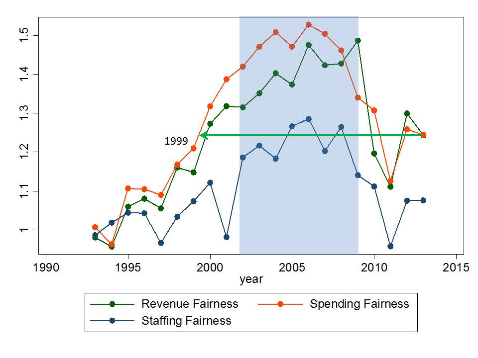
Whether the “money doesn’t matter” echo chamber is partly to blame, as the economy has begun to rebound in many states, school finance systems have become increasingly inequitable, with levels of state support for public schools stagnant at best (Leachman & Mai, 2014). The recent recession yielded an unprecedented decline in public school funding fairness [targeting of funds to high poverty districts]. Thirty-six states had a three year average reduction in current spending fairness between 2008-09 and 2010-11 and 32 states had a three year average reduction in state and local revenue fairness over that same time period (Baker, 2014b). A more recent report from the Center on Budget and Policy Priorities revealed that through 2014-15, most state school finance systems had not yet begun to substantively rebound (Leachman & Mai, 2014).

In short, the decline of state school finance systems continues and the rhetoric opposing substantive school finance reform shows little sign of easing. Districts serving the neediest student populations continue to take the hardest hit. Yet, concurrently, many states are raising outcome standards for students (Bandeira de Mello et al., 2015) and increasing the consequences on schools and teachers for not achieving those outcome standards. States are asking schools to do more with less, not knowing whether resources were sufficient to begin with, and states are asking schools to achieve equitable, high outcomes, with inequitable resources.

Recent Literature on School Finance Reforms

The growing political consensus that money doesn’t matter stands in sharp contrast to the substantial body of empirical research that has accumulated over time, but which gets little if any attention in our public discourse (Baker and Welner, 2011). From 2014 through 2015, Kirabo Jackson, Rucker Johnson and Claudia Persico released a series of papers (NBER working papers) and articles summarizing their analyses of a uniquely constructed national data set in which they evaluate the long term effects of selective, substantial infusions of funding to local public school districts which occurred primarily in the 1970s and 1980s, on high school graduate rates and eventual adult income (Jackson, Johnson and Persico, 2015a). Virtues of the JJP analysis include that the analysis provides clearer linkages than many prior studies between the mere presence of “school finance reform,” the extent to which school finance reform substantively changed the distribution of spending and other resources across schools and children, and the outcome effects of those changes. The authors also go beyond the usual, short run connections between changes in the level and distribution of funding, and changes in the level and distribution of test scores, to evaluate changes in the level and distribution of educational attainment, high school completion, adult wages, adult family income, and the incidence of adult poverty.

To do so, the authors use data from the Panel Study of Income Dynamics, on “roughly 15,000 PSID sample members born between 1955 and 1985, who have been followed into adulthood through 2011.” The authors analysis rests on the assumption that these individuals, and specific individuals among them, were differentially affected by the infusions of resources resulting from school finance reforms which occurred during their years in K-12 schooling. One methodological shortcoming of this long term analysis is the imperfect connection between the treatment and the population that received that treatment.[1] The authors matched childhood address data to school district boundaries to identify whether a child attended a district likely subject to additional funding as a result of court-mandated school finance reform. While imperfect, this approach creates a tighter link between the treatment and the treated than exists in many prior national, longitudinal, or even state specific school finance analyses (Baker and Welner, 2011a).

Regarding the effects of school finance reforms on long term outcomes, the authors summarize their major findings as follows:

Thus, the estimated effect of a 22 percent increase in per-pupil spending throughout all 12 school-age years for low-income children is large enough to eliminate the education gap between children from low-income and non-poor families. In relation to current spending levels (the average for 2012 was $12,600 per pupil), this would correspond to increasing per-pupil spending permanently by roughly $2,863 per student.

Specifically, increasing per-pupil spending by 10 percent in all 12 school-age years increases the probability of high school graduation by 7 percentage points for all students, by roughly 10 percentage points for low-income children, and by 2.5 percentage points for nonpoor children.

For children from low-income families, increasing per-pupil spending by 10 percent in all 12 school-age years boosts adult hourly wages by $2.07 in 2000 dollars, or 13 percent (see Figure 4).

The JJP study is not the only study which shows such gains. It just happens to be the most recent, and first in a long time (since Card and Payne, 2002) high profile national study of its kind. As discussed in a 2012 report from the Shanker Institute, numerous other researchers have explored the effects of specific state school finance reforms over time (Figlio, 2004). Several such studies provide compelling evidence of the potential positive effects of school finance reforms. Studies of Michigan school finance reforms in the 1990s have shown positive effects on student performance in both the previously lowest spending districts (Roy, 2011), and previously lower performing districts (Hyman, 2013, Papke, 2005). Similarly, a study of Kansas school finance reforms in the 1990s, which also involved primarily a leveling up of low-spending districts, found that a 20 percent increase in spending was associated with a 5 percent increase in the likelihood of students going on to postsecondary education (Deke, 2003).

Three studies of Massachusetts school finance reforms from the 1990s found similar results. The first, by Thomas Downes and colleagues found that the combination of funding and accountability reforms “has been successful in raising the achievement of students in the previously low-spending districts.” (Downes, Zabel & Ansel, 2009, p. 5) The second found that “increases in per-pupil spending led to significant increases in math, reading, science, and social studies test scores for 4th- and 8th-grade students.”(Guryan, 2001) The most recent of the three, published in 2014 in the Journal of Education Finance, found that “changes in the state education aid following the education reform resulted in significantly higher student performance.”(Nguyen-Hoang & Yinger, 2014, p. 297) Such findings have been replicated in other states, including Vermont.

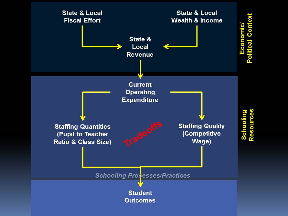
JJP also address the question of how money is spent. An important feature of the JJP study is that it does explore the resultant shifts in specific schooling resources in response to shifts in funding. For the most part, increased spending led to increases in typical schooling resources including higher salaries, smaller classes and longer days and years. JJP explain:

We find that when a district increases per-pupil school spending by $100 due to reforms, spending on instruction increases by about $70, spending on support services increases by roughly $40, spending on capital increases by about $10, while there are reductions in other kinds of school spending, on average.

We find that a 10 percent increase in school spending is associated with about 1.4 more school days, a 4 percent increase in base teacher salaries, and a 5.7 percent reduction in student-teacher ratios. Because class-size reduction has been shown to have larger effects for children from disadvantaged backgrounds, this provides another possible explanation for our overall results.

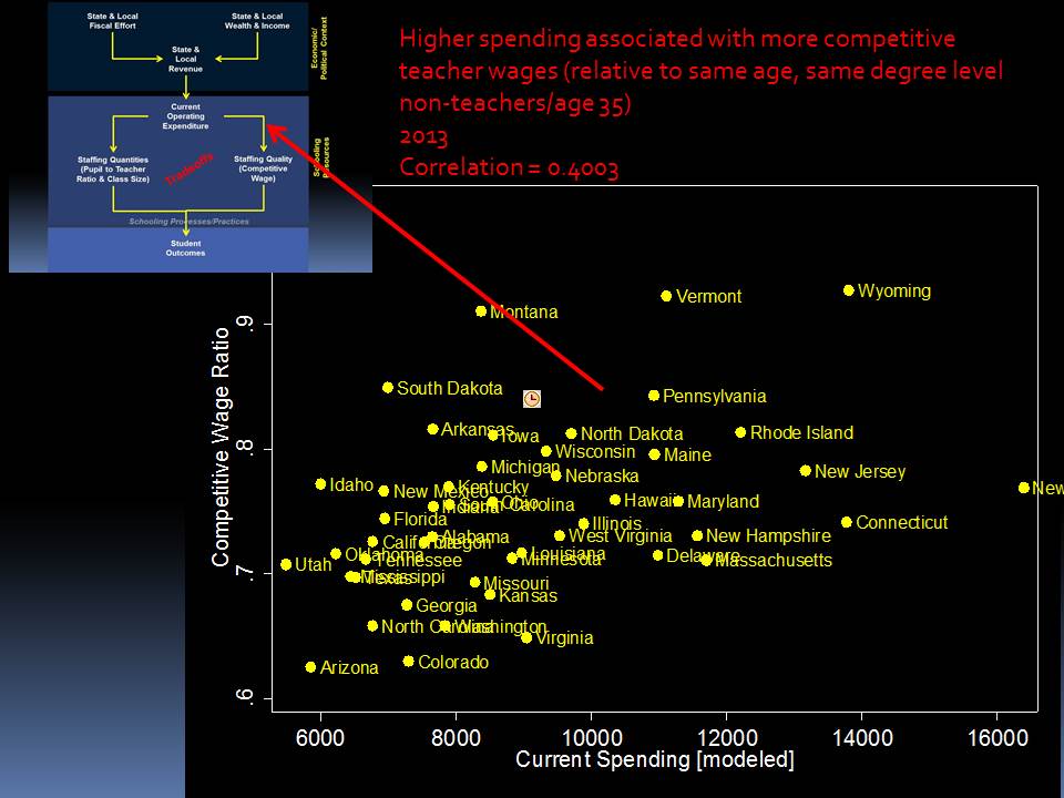
While there may be other mechanisms through which increased school spending improves student outcomes, these results suggest that the positive effects are driven, at least in part, by some combination of reductions in class size, having more adults per student in schools, increases in instructional time, and increases in teacher salaries that may help to attract and retain a more highly qualified teaching workforce.

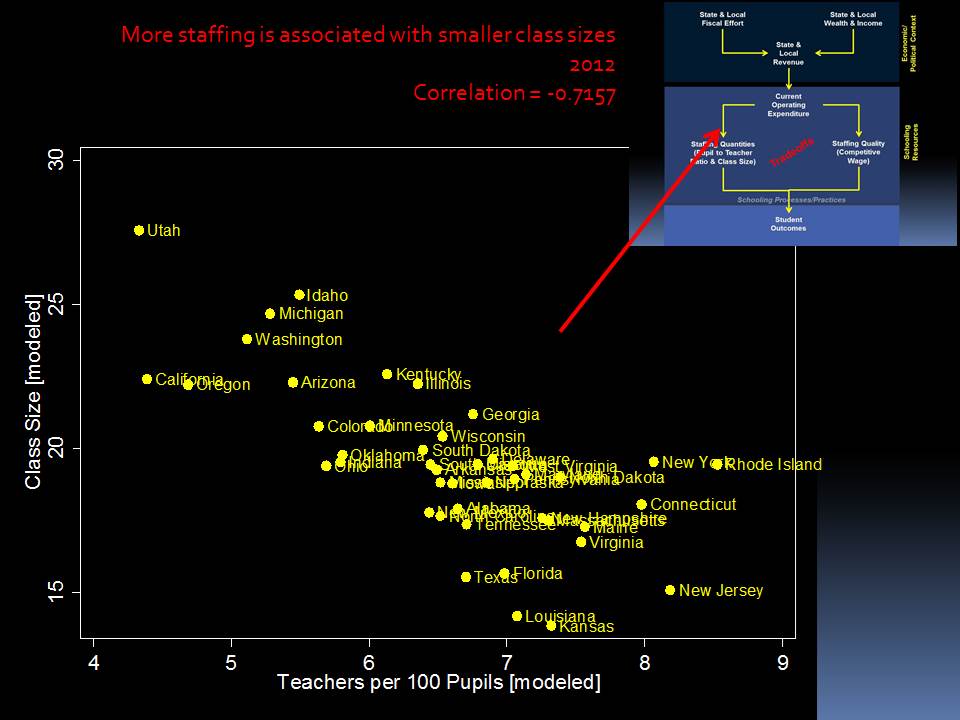
In other words, oft-maligned traditional investments in schooling resources occurred as a result of court imposed school finance reforms, and those changes in resources were likely responsible for the resultant long term gains in student outcomes. Such findings are particularly consistent with recent summaries and updated analyses of data on class size reduction.

Recent National Trends in Schooling Resources

The figures here illustrate recent trends in education spending and staffing. The echo chamber tells us that education spending has grown dramatically for decades, doubling if not tripling over time, and that staffing has expanded dramatically as well, with pupil to teacher ratios plummeting persistently to all-time lows in recent years.[2] Concurrently, the echo chamber mantra asserts that NAEP scores have been “virtually flat,”(which they have not)[3]

Figure 1 shows that over the 21 year period explored herein, spending is up about $400, or about 6.1% over the entire period, and up only $200, or about 2.6% from 2003 to 2013.

Figure 2 shows that elementary and secondary education spending as a share of personal income is lower than any time in the past decade and lower than 1993.

Further, while staffing ratios increased from 1993 to 2003, staffing ratios in 2013 had returned to levels similar to what they had been in 2000.

So, put bluntly, we have not continued to pour more and more resources into schools over the past decade (and then some). We have not put more and more effort into our spending on k12 public education systems – depleting our national or state economies.

Figure 1

Current Operating Expenditures per Pupil Adjusted for Labor Costs

Current Spending from U.S. Census Fiscal Survey of Local Governments (census.gov/govs/school). Labor cost adjustment from Taylor (Education Comparable Wage Index, at: http://bush.tamu.edu/research/faculty/taylor_CWI /)

Figure 2

Direct Education Expense as a Share of Gross Domestic Product

State & Local Government Finance Data Query System. http://www.taxpolicycenter.org/slf-dqs/pages.cfm. The Urban Institute-Brookings Institution Tax Policy Center. Data from U.S. Census Bureau, Annual Survey of State and Local Government Finances, Government Finances, Volume 4, and Census of Governments (Years). Date of Access: (09-Dec-15 08:31 AM)

Figure 3

Teachers per 100 Pupils

Staffing data from NCES Common Core of Data, Public Education Agency Universe Survey (nces.ed.gov/ccd).

Closing Thoughts

As I’ve explained on recent posts:

Accomplishing higher outcome goals will cost more, not less than past school spending, and doing so with increasingly needy student populations even more.

But the current approach in public policy is to expect more while providing less. And perhaps even more offensive, to expect the same higher outcomes across children and settings while providing and/or permitting vastly inequitable resources (and then to malign and punish those lacking sufficient resources to get the job done).

Dominant reform strategies (restructuring teacher compensation, or “chartering”) may by the most generous analysis, provide opportunity for small gains in efficiency, though many of those gains may not be sustainable/scalable and some may exacerbate inequities.

Further, the above trends represent national averages over time and mask substantial variation both across states and across districts and schools within states. As we move further toward common standards and assessments across states, consequences of substantial variations in access to resources will likely become more apparent.

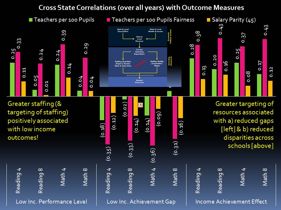
I will discuss in future posts how a) variations in the level of funding available in low income districts across states are associated with variations in the level of NAEP outcomes of those children across states and b) how the extent to which funding is targeted to lower income settings is associated with the extent to which NAEP outcome gaps are mitigated.

As I’ve explained previously, inequalities of education resources across settings matter greatly. Proclamations that Moneyball provides the solution for mitigating our nation’s achievement gaps are a cruel (and ignorant) joke.

Pondering Chartering: On Market Forces & Innovation?

One of the original premises of chartering as a competitive market tool was that introducing independently governed competitors and relaxing regulations on those competitors would induce innovation, which could then be shared for the good of the whole. This premise is flawed on many levels.

First, if innovation is to be induced by competition, there exists no incentive for competitors to share their innovations.

Second, if one subset of competitors is granted relaxation of regulations such that they can innovate, then that subset of competitors is granted an unfair advantage in that the regulations imposed on their competition (“district” schools) may inhibit their ability to “counter-innovate.”

Further, this system creates an incentive for the unregulated competitors to lobby for even stiffer regulation on their competition (“district” schools). [for example, lobbying in favor of test-driven teacher evaluation requirements to be imposed on “district” schools in a climate of public concern over the influence of testing – and then seeking exemption from those requirements for charter schools]

Of course, as I explained on a previous post, from ongoing writings, growth of the charter sector is hardly based on a competitive market model in the first place. Rather, that growth in many markets is already built on aggressive lobbying and manipulation of public policy:

It is important to acknowledge that charter school market shares are not, in recent years, expanding exclusively or even primarily because of market demand and personal/family preferences for charter schools. Traditional district public schools are being closed, neighborhoods left without options other than charters, district schools are being reconstituted and handed over to charter operators (including entire districts), and district schools are increasingly deprived of resources, experience burgeoning class sizes, reductions in program offerings sending more families scrambling for their “least bad” nearest alternative. [i] These are conscious decisions of policymakers overseeing the system that includes district and charter schools. They are not market forces, and should never be confused as such. These systems are being centrally managed without regard for equity and adequacy goals or the protection of student, family, taxpayer and employee rights, but instead, on the false hope that liberty of choice is a substitute for all of the above (including, apparently, loss of individual liberties). [ii]

Further, for all the talk that this model of competition (which really isn’t) would yield innovations not previously conceived, a growing body of research, including that most favorable to the charter sector suggests that truly novel innovations are hard to come by. Again from ongoing work:

While charter schooling was conceived as a way to spur innovation – try new things – evaluate them – and inform the larger system, studies of the structure and practices of charter schooling find the sector as a whole not to be particularly “innovative.” [iii] Analyses by charter advocates at the American Enterprise Institute find that the dominant form of specialized charter school is the “no excuses” model – a model which combines traditional curriculum and direct instruction with strict disciplinary policies and school uniforms, in some cases providing extended school days and years.[iv] Further, charter schools raising substantial additional revenue through private giving tend to use that funding to a) provide smaller classes, and b) pay teachers higher salaries for working longer days and years.[v] For those spending less, total costs are held down, when necessary, through employing relatively inexperienced, low wage staff and maintaining high staff turnover rates.[vi] In other words, the most common innovations are not especially innovative or informative for systemic reform.

Which leads me further down the road that we really need to rethink this “chartering” thing!

Notes

[i] See, for example:

Mezzacappa, Dale (2015, Oct. 1) Hite Plan: More charter conversions, closings, turnarounds, and new schools. Philadelphia Public School Notebook. http://thenotebook.org/blog/159023/hite-plan-more-renaissance-charters-closings-turnarounds-new-schools

Weber, Mark (2015) Empirical Critique of “One Newark”: First Year Update. New Jersey Education Policy Forum. https://njedpolicy.files.wordpress.com/2015/03/weber-testimony.pdf

Weber, Mark (2015, Jun. 5) Camden’s “Transformation” Schools: Racial & Experience Disparity in Staff Consequences. https://njedpolicy.files.wordpress.com/2015/06/weber_camdentransformationsfinal.pdf

[ii] Green, P.C.; & Baker, B.D.; & Oluwole, J. (2015, forthcoming). The Legal Status of Charter Schools in State Statutory Law- University of Massachusetts Law Review.

Green, P.C., Baker, B. D., & Oluwole, J.O. (2013). Having it both ways: How charter schools try to obtain funding of public schools and the autonomy of private schools. Emory Law Journal, 63, 303-337.

Mead, J.F. (2015). The Right to an Education or the Right to Shop for Schooling: Examining Voucher Programs in Relation to State Constitutional Guarantees, 42 Fordham Urban Law Journal 703.

Civil Rights Suspended: An Analysis of New York City Charter School Discipline Policies (2015). Advocates for Children of New York. http://www.advocatesforchildren.org/sites/default/files/library/civil_rights_suspended.pdf?pt=1

[iii] Preston, C., Goldring, E., Berends, M., & Cannata, M. (2012). School innovation in district context: Comparing traditional public schools and charter schools. Economics of Education Review, 31(2), 318-330.

[iv] Michael Q. McShane and Jenn Hatfield (2015) Measuring Diversity in Charter School Offerings. Washington, DC: American Enterprise Institute. http://www.aei.org/wp-content/uploads/2015/07/Measuring-Diversity-in-Charter-School-Offerings.pdf

[v] Baker, B. D., Libby, K., & Wiley, K. (2012). Spending by the Major Charter Management Organizations: Comparing Charter School and Local Public District Financial Resources in New York, Ohio, and Texas. National Education Policy Center.

[vi] Epple, D., Romano, R., & Zimmer, R. (2015). Charter schools: a survey of research on their characteristics and effectiveness (No. w21256). National Bureau of Economic Research.

Toma, E., & Zimmer, R. (2012). Two decades of charter schools: Expectations, reality, and the future. Economics of Education Review, 31(2), 209-212.

At the Intersection of Money & Reform Part III: On Cost Functions & the Increased Costs of Higher Outcomes

In my 2012 report Does Money Matter in Education, I addressed the education production function literature that seeks to establish a direct link between resources spent on schools and districts, and outcomes achieved by students. Production function studies include studies of how variation in resources across schools and settings is associated with variations in outcomes across those settings, and whether changes in resources lead to changes in the level or distribution of outcomes.

I have written previously on this blog about the usefulness of education cost functions.

The Education Cost Function

The education cost function is the conceptual flip side of the education production function. Like production function research, cost function research seeks to identify the link between spending variation and outcome variation, cross-sectionally and longitudinally. The goal of the education cost function is to discern the levels of spending associated with efficiently producing specific outcome levels (the “cost” per se) across varied geographic contexts and schools serving varied student populations. Most published studies applying cost function methodology use multiple years of district-level data, within a specific state context, and focus on the relationship between cross-district (over time) variations in spending and outcome levels, considering student characteristics, contextual characteristics such as economies of scale, and labor cost variation. Districts are the unit of analysis because they are the governing unit charged with producing outcomes, raising and receiving the revenues, and allocating the financial and human resources for doing so. Some cost function studies evaluate whether varied expenditures are associated with varied levels of outcomes, all else being equal, while other cost function studies evaluate whether varied expenditures are associated with varied growth in outcomes.

The existing body of cost function research has produced the following (in some cases obvious) findings:

The per-pupil costs of achieving higher-outcome goals tend to be higher, across the board, than the costs of achieving lower-outcome goals, all else being equal.[1]
The per-pupil costs of achieving any given level of outcomes are particularly sensitive to student population characteristics. In particular, as concentrated poverty increases, the costs of achieving any given level of outcomes increase significantly.[2]
The per-pupil costs of achieving any given level of outcomes are sensitive to district structural characteristics, most notably, economies of scale.[3]

Researchers have found cost functions of particular value for evaluating the different costs of achieving specific outcome goals across settings and children. In a review of cost analysis methods in education, Downes (2004) explains: “Given the econometric advances of the last decade, the cost-function approach is the most likely to give accurate estimates of the within-state variation in the spending needed to attain the state’s chosen standard, if the data are available and of a high quality” (p. 9).[4]

Addressing the critics

This body of literature also has its detractors, including, most notably, Robert Costrell, Eric Hanushek and Susanna Loeb (CHL), who, in a 2008 article, assert that cost functions are invalid for estimating costs associated with specific outcome levels. They assert that one cannot possibly identify the efficient spending level associated with achieving any desired outcome level by evaluating the spending behavior of existing schools and districts, whose spending is largely inefficient (because, as discussed above, district expenditures are largely tied up in labor agreements that, according to these authors, are in no way linked to the production of student outcomes). If all schools and districts suffer such inefficiencies, then one cannot possibly discern underlying minimum costs by studying those institutions. However, CHL’s argument rests on the assumption that desired outcomes could be achieved while spending substantially less and entirely differently than any existing school or district spends, all else being equal. Evidence to this effect is sparse to nonexistent.[5]

Authors of cost function research assert, however, that the goal of cost modeling is more modest than exact predictions of minimum cost, and that much can be learned by better understanding the distribution of spending and outcomes across existing schools and districts, and the varied efficiency with which existing schools and districts achieve current outcomes.[6] That is, the goal of the cost model is to identify, among existing “outcome producing units” (districts or schools), the more (and less) efficient spending levels associated with given outcomes, where those more efficient spending levels associated with any given outcome provide a real-world approximation, approaching the minimum costs of achieving those outcomes.

CHL’s empirical critique of education cost function research centers on a falsification test, applying findings from a California study by Jennifer Imazeki (2008).[7] CHL’s critique was published in a non-peer-reviewed special issue of the Peabody Journal of Education, based on testimony provided in the state of Missouri and funded by the conservative Missouri-based Show-Me Institute.[8] The critique asserts that if, as it would appear conceptually, the cost function is merely the flip side of the production function, then the magnitude of the spending-to-outcomes relationship should be identical between the cost and production functions. But, in Imazeki’s attempt to reconcile cost and production functions using California data, the results differed dramatically. That is, if one uses a production function to identify the spending associated with certain outcome levels, and then the cost function, the results differ dramatically. CHL use this finding to assert the failure of cost functions as a method and, more generally, the uncertainty of the spending-to-outcomes relationship.

Duncombe and Yinger (2011), however, explain the fallacy of this falsification test, in a non-peer-reviewed special issue of the same journal.[9] They explain that while the cost and production functions are loosely flip sides of the same equation, they are not exactly such. Production models are estimated using some outcome measure as the dependent variable—that which is predicted by the equation. In an education production function studying the effect of spending on outcomes, the dependent variable is predicted as a function of (a) a measure of relevant per-pupil spending; (b) characteristics of the student population served; and (c) contextual factors that might affect the value of the dollar toward achieving outcomes (economies of scale, regional wage variation).

Outcomes = f(Spending, Students, Context)

The cost model starts out similarly, switching the position of the spending and outcomes measures, and predicting spending levels as a function of outcomes, students and context factors.

Spending = f(Outcomes, Students, Context)

If it was this simple, then one would expect the statistical relationship between outcomes and spending to be the same from one equation to the next. But there’s an additional piece to the cost function that, in fact, adds important precision to the estimation of the input to outcome relationship. The above equation is a spending function, whereas the cost function attempts to distill “cost” from spending by addressing the share of spending that may be “inefficient.” That is:

Cost = Spending – Inefficiency, or Spending = Cost + Inefficiency

That is, some of the variation in spending is variation that does not lead to variations in the outcome measure. While we don’t really know exactly what the inefficiency is (which dollars are being spent in ways that don’t improve outcomes), Duncombe and Yinger suggest that we do know some of the indirect predictors of the likelihood that school districts spend more than would be needed to minimally achieve current outcomes, and that one can include in the cost model characteristics of districts that explain a portion of the inefficient spending. This can be done when the spending measure is the dependent variable, as in the cost function, but not when the spending variable is an independent measure, as in the production function.[10]

Spending = f(Outcomes, Students, Context, Inefficiency Factors)

When inefficiency factors are accounted for in the spending function, the relationship between outcomes and spending more accurately represents a relationship between outcomes and costs. This relationship would be expected to be different from the relationship between spending and outcomes (without addressing inefficiency) in a typical production function.

In Summary

In summary, while education cost function research is not designed to test specifically whether and to what extent money matters, the sizeable body of cost function literature does suggest that achieving higher educational outcomes, all else being equal, costs more than achieving lower educational outcomes. Further, achieving common educational outcome goals in settings with concentrated child poverty, children for whom English is a second language and children with disabilities costs more than achieving those same outcome goals with less needy student populations. Cost models provide some insights into how much more money is required in different settings and with different children to achieve measured outcome goals. Such estimates are of particular interest in this period of time when more and more states are migrating toward common standards frameworks and common assessments but are still providing their schools and districts with vastly different resources. Cost modeling may provide insights into just how much more funding may be required for all children to have equal opportunity to achieve these common outcome goals.

Notes

[1]W. Duncombe and J. Yinger, “Financing Higher Student Performance Standards: The Case of New York State,” Economics of Education Review 19, no. 4 (2000): 363-386; A. Reschovsky and J. Imazeki, “Achieving Educational Adequacy through School Finance Reform,” Journal of Education Finance (2001): 373-396;
J. Imazeki and A. Reschovsky, “Is No Child Left Behind an Un (or Under) Funded Federal Mandate? Evidence from Texas,” National Tax Journal (2004): 571-588; J. Imazeki and A. Reschovsky, “Does No Child Left Behind Place a Fiscal Burden on States? Evidence from Texas,” Education Finance and Policy 1, no. 2 (2006): 217-246; and J. Imazeki and A. Reschovsky, “Assessing the Use of Econometric Analysis in Estimating the Costs of Meeting State Education Accountability Standards: Lessons from Texas,” Peabody Journal of Education 80, no. 3 (2005): 96-125.

[2]T. A. Downes and T. F. Pogue, “Adjusting School Aid Formulas for the Higher Cost of Educating Disadvantaged Students,” National Tax Journal (1994): 89-110; W. Duncombe and J. Yinger, “School Finance Reform: Aid Formulas and Equity Objectives,” National Tax Journal (1998): 239-262; W. Duncombe and J. Yinger, “Why Is It So Hard to Help Central City Schools?,” Journal of Policy Analysis and Management 16, no. 1 (1997): 85-113; and W. Duncombe and J. Yinger, “How Much More Does a Disadvantaged Student Cost?,” Economics of Education Review 24, no. 5 (2005): 513-532.

[3]For a discussion, see B. D. Baker, “The Emerging Shape of Educational Adequacy: From Theoretical Assumptions to Empirical Evidence,” Journal of Education Finance (2005): 259-287. See also M. Andrews, W. Duncombe and J. Yinger, “Revisiting Economies of Size in American Education: Are We Any Closer to a Consensus?,” Economics of Education Review 21, no. 3 (2002): 245-262; W. Duncombe, J. Miner and J. Ruggiero, “Potential Cost Savings from School District Consolidation: A Case Study of New York,” Economics of Education Review 14, no. 3 (1995): 265-284; J. Imazeki and A. Reschovsky, “Financing Adequate Education in Rural Settings,” Journal of Education Finance (2003): 137-156; and T. J. Gronberg, D. W. Jansen and L. L. Taylor, “The Impact of Facilities on the Cost of Education,” National Tax Journal 64, no. 1 (2011): 193-218.

[4]T. Downes, What Is Adequate? Operationalizing the Concept of Adequacy for New York State (2004), http://www.albany.edu/edfin/Downes%20EFRC%20Symp%2004%20Single.pdf.

[5] For a recent discussion, see: Baker, B., & Welner, K. G. (2012). Evidence and rigor scrutinizing the rhetorical embrace of evidence-based decision making. Educational Researcher, 41(3), 98-101. See also: Baker, B. D. (2012). Revisiting the Age-Old Question: Does Money Matter in Education?. Albert Shanker Institute.

[6]See, for example, B. D. Baker, “Exploring the Sensitivity of Education Costs to Racial Composition of Schools and Race-Neutral Alternative Measures: A Cost Function Application to Missouri,” Peabody Journal of Education 86, no. 1 (2011): 58-83.

[7]Completed and released in 2006, eventually published as J. Imazeki, “Assessing the Costs of Adequacy in California Public Schools: A Cost Function Approach,” Education 3, no. 1 (2008): 90-108.

[8]See the acknowledgements at http://files.eric.ed.gov/fulltext/ED508961.pdf. Final published version: R. Costrell, E. Hanushek and S. Loeb, “What Do Cost Functions Tell Us about the Cost of an Adequate Education?,” Peabody Journal of Education 83, no. 2 (2008): 198-223.

[9]W. Duncombe and J. Yinger, “Are Education Cost Functions Ready for Prime Time? An Examination of Their Validity and Reliability,” Peabody Journal of Education 86, no. 1 (2011): 28-57. See also W. Duncombe and J. M. Yinger, “A Comment on School District Level Production Functions Estimated Using Spending Data” (Maxwell School of Public Affairs, Syracuse University, 2007); and W. Duncombe and J. Yinger, “Making Do: State Constraints and Local Responses in California’s Education Finance System,” International Tax and Public Finance 18, no. 3 (2011): 337-368. For an alternative approach, see T. J. Gronberg, D. W. Jansen and L. L. Taylor, “The Adequacy of Educational Cost Functions: Lessons from Texas,” Peabody Journal of Education 86, no. 1 (2011): 3-27.

[10]W. Duncombe and J. Yinger, “Are Education Cost Functions Ready for Prime Time? An Examination of Their Validity and Reliability,” Peabody Journal of Education 86, no. 1 (2011): 28-57. See also W. Duncombe and J. M. Yinger, “A Comment on School District Level Production Functions Estimated Using Spending Data” (Maxwell School of Public Affairs, Syracuse University, 2007). For an alternative approach, see T. J. Gronberg, D. W. Jansen and L. L. Taylor, “The Adequacy of Educational Cost Functions: Lessons from Texas,” Peabody Journal of Education 86, no. 1 (2011): 3-27.

Pondering Chartering: Getting the incentives right for the good of the whole!

I had a fun chat with EduShyster the other day about my recent report on charter school business practices. It was during the course of that conversation that I articulated some of my major concerns about how we are currently approaching “chartering” as public policy, and, for that matter, academic researchers of chartering as public policy. Here are a few points that I think are key takeaways from my recent ramblings.

First, I discuss the fact that there are “better” and “worse” actors in the present system. But a major problem is that there’s little pressure for anyone to do anything about the “worse” actors (or “bad apples” as Edushyster called them). I explained:

It’s to the benefit of the good guys to have the bad guys there because it makes them look better. When you’re KIPP, you look that much better when White Hat does something awful.

Further, because we (including policy researchers) are obsessed with what I refer to as “pissing match” studies of whether charter schools on average “outperform” matched, district, or schools of “lotteried out” kids, it’s in the interest of charter operators to gain every edge they can over the “competition” (or the “comparison” group, or “counterfactual”). In other words, it’s NOT in their interest to support strengthening the “competition.” I explained:

It’s just like the way that they continually argue for boosting their own subsidy, even if they know full well it’s at the expense of the district.

The problem is that there’s no incentive under the current policy structure for them to want the district schools to do better. And there’s every incentive for them not to. That’s what’s wrong with this system. Even when they’re good folks and trying to do a good thing, there’s still that undercurrent.

It’s time for all of us to rethink how we frame this conversation to get the incentives right!

Pondering Chartering: What do we know about administrative and instructional spending?

In a recent report, Gary Miron and I discuss some of the differences in resource allocation practices between Charter operators and district schools. Among other things, we discuss the apparently high administrative expenses of charter operators. But in that same report, we explain that some of these higher administrative expenses, and, as a result lower instructional expenses, result from bad policy structures that constrain resource allocation and/or induce seemingly illogical behaviors.

Some have pointed out to me that this assertion of higher administrative and lower instructional expense by charter operators runs counter claims made by Dale Russakoff in her book The Prize. My doc student Mark Weber has already thoroughly rebutted Russakoff’s anecdotal claims. Put bluntly. Those claims were supported only by anecdote and run in contrast with the larger body of data in New Jersey (see Mark’s post) and larger literature on the topic. The summary below addresses additional literature on this topic.

[to be clear… and this is a topic for another post, or perhaps Matt Barnum will do a piece on this… there is little if any evidence that administrative expense shares alone are an indicator if “inefficiency,” where inefficiency is defined as a reduction in outcomes produced for the same aggregate dollar input]

In a related recent post, I explain whether “chartering” can tell us much/anything about whether and how money (and resources that cost money) are associated with measured student outcomes.

Below is a section of a separate, forthcoming paper (coauthored with Mark Weber), in which we evaluate school site staffing expenditure differences between district, non-profit and for-profit charter operators.

Charter School Administrative/Instruction Expense

A handful of studies over time have addressed questions similar to those we address herein, asking more specifically about the differences in administrative overhead expenditures of charter schools. Two studies of Michigan charter schools, which operate fiscally independently of local public districts, have found them to have particularly high administrative expenses and low direct instructional expenses. Arsen and Ni (2012) found that “Controlling for factors that could affect resource allocation patterns between school types, we find that charter schools on average spend $774 more per pupil per year on administration and $1141 less on instruction than traditional public schools.” (p. 1) Further, they found “charter schools managed by EMOs spend significantly more on administration than self-managed charters (about $312 per pupil). This higher spending occurs in administrative functions traditionally performed at both the district central office and school building levels.” (p. 13)

Izraeli and Murphy (2012) found that district schools in Michigan tended to spend more on instruction per student than did charter schools, and the gap grew by about 5 percent to nearly 35% percent over the period studied (1995-96 to 2005-06) (p. 265). Further they found the spending gap for instructional spending to be greater than that for general spending. The overall funding gap between district and charter schools was approximately $230. The spending gap for basic programs was $562 and for total instruction $910. The authors note “much like a profit-maximizing firm, charter schools generate a surplus of revenue over expenditure.” (Izraeli & Murphy, 2012, p. 265)

Bifulco and Reback (2014) explore the complex relationship between fiscally dependent charter schools and their host districts in upstate New York cities. Particularly relevant to our investigation is Bifulco and Reback’s finding that having fiscally dependent charter schools separately affiliated with outside management companies and governance structures can create excess, redundant costs (p. 86).

Others have explored teacher compensation in relation to instructional expense in charter schools. In a recent comprehensive review of charter school research, Epple, Romano and Zimmer (2015) summarize that “On the whole, teachers in charter schools are less experienced, are less credentialed, are less white, and have fewer advanced degrees. They are paid less, their jobs are less secure, and they turnover with higher frequency.” (Epple, 2015) Similarly, in a report on spending behavior of Texas charter schools Taylor and colleagues (2011) explain that much of the difference between instructional and non-instructional expense across differing types of charter and district schools is tied to differences in teacher compensation. The authors explain that “open-enrollment charter schools paid lower salaries, on average, than did traditional public school districts. Average teacher pay was 12% lower for teachers in open-enrollment charter schools than for teachers in traditional public school districts of comparable size, and adjusted for differences in local wage levels, average teacher pay was 24% lower. Average teacher salaries were lower not only because open-enrollment charter schools hired less experienced teachers, on average, but also because open-enrollment charter schools paid a smaller premium for additional years of teacher experience.” (p. ix)

Research by Gronberg, Taylor and Jansen (2012) also points to the revenue enhancement activities of some charter management companies, most notably KIPP schools. The authors find that some KIPP schools in Texas had nearly doubled their per pupil public subsidy through private philanthropy. Baker and Ferris (2011) and Baker, Libby and Wiley (2012, 2015) find similarly that some Charter Management Organizations have significant potential for revenue enhancement. Baker, Libby and Wiley (2012) explain “We find that in New York City, KIPP, Achievement First and Uncommon Schools charter schools spend substantially more ($2,000 to $4,300 per pupil) than similar district schools. Given that the average spending per pupil was around $12,000 to $14,000 citywide, a nearly $4,000 difference in spending amounts to an increase of some 30%.” But, while some New York City based CMOs raised substantial private funding, others did not, and charter schools operating in other locations in Ohio and Texas had much less access to philanthropy.

Relative Efficiency & Underlying Differences

Of particular interest herein are studies of the relative effectiveness or efficiency of charter schools operated by for-profit management companies, including operators of online schools. Rigorous, peer reviewed literature on these schools remains limited, and much of it dated, evaluating charter expansion from the late 1990s through mid-2000s. King (2007) evaluated the effectiveness of Arizona charter schools, where there exist significant numbers of for profit firms. King (2007) found, based on data from 2003-2004 that “there is some evidence that for-profit charter schools are achieving higher test scores, however, given the insignificant findings for many of the for-profit specifications, a definite conclusion cannot be reached based on this one study alone. (King, 2007, p. 744) However, in a broader, more recent and more empirically rigorous analysis of Arizona charter schools as a whole Chingos and West (2014) found that “the performance of charter schools in Arizona in improving student achievement varies widely, and more so than that of traditional public schools. On average, charter schools at every grade level have been modestly less effective than traditional public schools in raising student achievement in some subjects.” (p. 120S)

Studies on Michigan charter schools, another state we identify has having significant shares of children enrolled in for-profit schools, have also yielded mixed findings over time regarding effectiveness and relative efficiency. Bettinger (2005) found that during the early years of Michigan charter schools, “test scores of charter school students do not improve, and may actually decline, relative to those of public school students.” (p. 133) Hill and Welsch (2009) found “no evidence of a change in efficiency when a charter school is run by a for-profit company (versus a not-for-profit company). (p. 147) They explain further: “The results of this paper find no evidence that schools managed by for-profit companies deliver education services less efficiently than schools run by not-for-profit companies; this matches recent results found by Sass (2006).” (p. 164) That is, the shift from nonprofit to for-profit management status caused no systematic harm to measured student outcomes. Sass (2004) in an early study of Florida charter schools by their management status had also found no significant performance differences between schools managed by nonprofit and for-profit providers, but had found that for-profit providers serve substantively fewer children with disabilities. (p. 91)

Perhaps the strongest evidence of charter school efficiency advantages comes from the work of Gronberg, Taylor and Jansen (2012) on Texas charter schools. The authors find that, generally, Texas “charter schools are able to produce educational outcomes at lower cost than traditional public schools—probably because they face fewer regulations—but are not systematically more efficient relative to their frontier than are traditional public schools.”(p. 302) In other words, while the overall cost of charter schools is lower for comparable output, the variations in relative efficiency among Texas charter schools are substantial. Efficiency is neither uniformly nor consistently achieved. As explained above, evidence from related work by these authors reveals that the lower overall expenses are largely a function of lower salaries and inexperienced staff (Taylor et al., 2011). Thus, maintaining efficiency may require ongoing reliance on inexperienced staff.

Frequently cited studies touting the relative effectiveness of charter schools operated by major Charter Management Organizations, including Lake et al. (2010) and Dobbie and Fryer (2011) have typically measured poorly or not at all the resources available in these schools – schools which Baker, Libby and Wiley (2015, 2012) and Gronberg, Taylor and Jansen (2012) identify as often spending substantially more than nearby district schools. Baker, Libby and Wiley (2015) and others (Preston et al., 2012) explain that most charter schools, and large CMO charter schools in particular, operate under a similar human resource intensive model as traditional district schools. Specifically, well-endowed CMOs allocate their additional resources to competitive wages (higher than expected for relatively inexperienced teachers), small classes, longer days and years (Baker, Libby and Wiley, 2012).

Other charter school operators have attempted to reduce substantially direct instructional per pupil costs through online and hybrid learning. This approach provides perhaps the greatest opportunity to maximize profit margin as it presents the greatest opportunity to cut staffing costs. But as Epple, Romano and Zimmer (2015) explain, regarding student outcomes “online ‘cyber’ schools appear to be a failed innovation, delivering markedly poorer achievement outcomes than TPSs.” (p. 55)

Pulling it All Together

To summarize, based on limited analyses of resource allocation behaviors of charter schools, we have evidence that charter schools generally tend to divert more from the classroom to administration. Classroom expenditures are reduced in part, if not mainly by reduction of total teacher salary expenses by having relatively inexperienced teachers and high turnover rates. EMO operated charter schools tend to have even greater administrative expense and charter schools operating within districts may create redundant administrative expenses. That said, there is limited evidence that charter schools generally, or those operated by EMOs and CMOs are less efficient as a result of increased administrative expense, and some evidence of efficiency improvement for charters over district schools (in Texas) due to reduced staffing expenditure. Generally, we have little evidence of systematic differences between nonprofit and for-profit operated charter schools, but we do have some evidence that high profile nonprofit providers engage in substantial revenue enhancement. Finally, we have increasingly clear evidence that online and cyber charter schools lag in performance outcomes, as well as evidence that charter schools in states including Ohio and Arizona perform particularly poorly.

References

Andrews, M., Duncombe, W., & Yinger, J. (2002). Revisiting economies of size in American education: are we any closer to a consensus?. Economics of Education Review, 21(3), 245-262.

Arsen, D. D., & Ni, Y. (2012). Is administration leaner in charter schools? Resource allocation in charter and traditional public schools. education policy analysis archives, 20, 31.

Baker, B.D. & Bathon, J. (2012). Financing Online Education and Virtual Schooling: A Guide for Policymakers and Advocates. Boulder, CO: National Education Policy Center. Retrieved 7/14/15 from http://nepc.colorado.edu/publication/financing-online-education

Baker, B. D., & Elmer, D. R. (2009). The politics of off-the-shelf school finance reform. Educational Policy, 23(1), 66-105.

Baker, B. D., & Ferris, R. (2011). Adding up the Spending: Fiscal Disparities and Philanthropy among New York City Charter Schools. National Education Policy Center.

Baker, B.D., Libby, K., Wiley, K. (2015) Charter School Expansion & Within District Equity: Confluence or Conflict? Education Finance and Policy

Baker, B. D., Libby, K., & Wiley, K. (2012). Spending by the Major Charter Management Organizations: Comparing Charter School and Local Public District Financial Resources in New York, Ohio, and Texas. National Education Policy Center.

Bettinger, E. P. (2005). The effect of charter schools on charter students and public schools. Economics of Education Review, 24(2), 133-147.

Bifulco, R., & Reback, R. (2014). Fiscal Impacts of Charter Schools: Lessons from New York. Education Finance & Policy, 9(1), 86-107.

Bitterman, A., Gray, L., and Goldring, R. (2013). Characteristics of Public and Private Elementary and Secondary Schools in the United States: Results From the 2011–12 Schools and Staffing Survey (NCES 2013–312). U.S. Department of Education. Washington, DC: National Center for Education Statistics. Retrieved 7/14/15 from https://nces.ed.gov/pubs2013/2013312.pdf

Bulkley, K. E., & Burch, P. (2011). The changing nature of private engagement in public education: For-profit and nonprofit organizations and educational reform. Peabody Journal of Education, 86(3), 236-251.

Center for Research on Education Outcomes (CREDO) (2013, June). National Charter School Study. Palo Alto: CREDO, Stanford University. Retrieved July 10, 2013, from http://credo.stanford.edu/research-reports.html

Chingos, M. M., & West, M. R. (2015). The Uneven Performance of Arizona’s Charter Schools. Educational Evaluation and Policy Analysis, 37(1 suppl), 120S-134S.

Dobbie, W., & Fryer Jr, R. G. (2011). Getting beneath the veil of effective schools: Evidence from New York City (No. w17632). National Bureau of Economic Research.

Duncombe, W., & Yinger, J. (2008). Measurement of cost differentials. Handbook of research in education finance and policy, 238-256.

Education Trust-Midwest (2015) Accountability for All: The need for real charter school authorizer accountability in Michigan. http://www.crainsdetroit.com/assets/PDF/CD98381219.PDF

Epple, D., Romano, R., & Zimmer, R. (2015). Charter Schools: A Survey of Research on Their Characteristics and Effectiveness (No. w21256). National Bureau of Economic Research.

Gronberg, T. J., Jansen, D. W., & Taylor, L. L. (2012). The relative efficiency of charter schools: A cost frontier approach. Economics of Education Review, 31(2), 302-317.

Hill, C. D., & Welsch, D. M. (2009). For‐profit versus not‐for‐profit charter schools: an examination of Michigan student test scores. Education Economics, 17(2), 147-166.

Izraeli, O., & Murphy, K. (2012). An Analysis of Michigan Charter Schools: Enrollment, Revenues, and Expenditures. Journal of Education Finance, 37(3), 234-266.

Kena, G., Musu-Gillette, L., Robinson, J., Wang, X., Rathbun, A., Zhang, J., Wilkinson-Flicker, S., Barmer, A., and Dunlop Velez, E. (2015). The Condition of Education 2015 (NCES 2015-144); p.85. U.S. Department of Education, National Center for Education Statistics. Washington, DC. Retrieved 7/14/15 from http://nces.ed.gov/pubs2015/2015144.pdf

King, K. A. (2007). Charter Schools in Arizona: Does Being a For-Profit Institution Make a Difference?. Journal of Economic Issues, 729-746.

Lake, R., Dusseault, B., Bowen, M., Demeritt, A., & Hill, P. (2010). The National Study of Charter Management Organization (CMO) Effectiveness. Report on Interim Findings. Center on Reinventing Public Education.

Maul, A., & McClelland, A. (2013). REVIEW OF NATIONAL CHARTER SCHOOL STUDY 2013. Boulder, CO: National Education Policy Center. Retrieved September, 2, 2014.

Maul, A. (2013). Review of “Charter School Performance in Michigan.”. Boulder, CO: National Education Policy Center. Retrieved July, 10, 2013.

Miron, G., & Gulosino, C. (2013). Profiles of for-profit and nonprofit education management organizations: Fourteenth Edition—2011-2012. Boulder, CO: National Education Policy Center.

Molnar, A., Huerta, L., Rice, J. K., Shafer, S. R., Barbour, M. K., Miron, G., … & Horvitz, B. (2014). Virtual Schools in the US 2014: Politics, Performance, Policy, and Research Evidence.

Morley, J. (2006). For-profit and nonprofit charter schools: An agency costs approach. The Yale Law Journal, 1782-1821.

Preston, C., Goldring, E., Berends, M., & Cannata, M. (2012). School innovation in district context: Comparing traditional public schools and charter schools. Economics of Education Review, 31, 318–330.

Richards, C. E. (1996). Risky Business: Private Management of Public Schools. Economic Policy Institute, 1660 L Street, NW, Suite 1200, Washington, DC 20036.

Sass, T. R. (2006). Charter schools and student achievement in Florida. Education Finance and Policy, 1(1), 91-122.

Taylor, L.L., and Fowler, W.J., Jr. (2006). A Comparable Wage Approach to Geographic Cost Adjustment (NCES 2006-321). U.S. Department of Education. Washington, DC: National Center for Education Statistics.

Taylor, L.L. Alford, B.L., Rollins, K.G., Brown, D.B., Stillisano. J.R., Waxman, H.C. (2011) Evaluation of Texas Charter Schools 2009-2010 (Revised Draft). Texas Education Research Center. Texas A&M University, College Station.

Zimmer, R., Gill, B., Booker, K., Lavertu, S., & Witte, J. (2012). Examining charter student achievement effects across seven states. Economics of Education Review, 31(2), 213-224.

Picture Post Week: Subprime Chartering

A short while back, I explained how, in our fervor to rapidly expand charter schooling and decrease the role of large urban school districts in serving their resident school-aged populations, we’ve created some particularly ludicrous scenarios whereby, for example – charter school operators use public tax dollars to buy land and facilities that were originally purchased with other public dollars… and at the end of it all, the assets are in private hands! Even more ludicrous is that the second purchase incurred numerous fees and administrative expenses, and the debt associated with that second purchase likely came with a relatively high interest rate because – well – revenue bonds paid for by charter school lease payments are risky. Or so the rating agencies say.

So how much of this debt is accumulating? And when does it come due? Who is issuing this debt? Are we looking at a charter school subprime bubble? Here are some snapshots:

Most revenue bond debt incurred on behalf of charter schools is either unrated, or BBB- or BB+ rated. The unrated debt is saddled, on average, with coupon rates around 6.9% in recent years, marginally higher than rates attached to BBB- or BB+ bonds.

PIMA County Industrial Development Authority in Arizona has been particularly active in recent years! Still trying to figure this one out.

So, are we at risk of a subprime chartering collapse?

What will happen to all of this debt if some of the bigger charter chains go belly up? Can’t make their (at times exorbitant) lease payments?

Have we let the charter industry get “too big to fail?” [certainly by comparison, this is a tiny bubble, but it’s really just getting started]

And when and how will that bail out occur? [and who will own those facilities when the dust settles?]

And just remember who’s running charter schools in the states where the debt is accumulating the fastest!

Picture Post Week: Increased Standards & Student Needs, But Shrinking Resources!

As I explain in a post a while back:

In short, the “cost” of education rises as a function of at least 3 major factors:

Changes in the incoming student populations over time
Changes in the desired outcomes for those students, including more rigorous core content area goals or increased breadth of outcome goals
Changes in the competitive wage of the desired quality of school personnel

And the interaction of all three of these! For example, changing student populations making teaching more difficult (a working condition), meaning that a higher wage might be required to simply offset this change. Increasing the complexity of outcome goals might require a more skilled teaching workforce, requiring higher wages.

So how well have we been addressing the increased costs associated with both our increasingly needy student populations, and our desire for higher outcome standards?

Not so well I guess!

Share this:

A little background

How related are variations in PARCC scores with variations in ASK scores across New Jersey schools?

How much does a PARCC proficiency cut score requirement of 750 raise (or lower) the bar when compared to an ASK proficiency cut score of 200?

Distributions of missing scores

Share this:

REALLY SIMPLE MODEL

INDICATORS

Financial Inputs

Real Resource Inputs

Outcome Levels and Disparities

PREVIEW OF CROSS STATE PATTERNS

Share this:

Recent Literature on School Finance Reforms

Recent National Trends in Schooling Resources

Share this:

Share this:

The Education Cost Function

Addressing the critics

In Summary

Share this:

Share this:

Charter School Administrative/Instruction Expense

Relative Efficiency & Underlying Differences

Pulling it All Together

References

Share this:

Share this:

Share this:

References

Baker, B.D. (2014) America’s Most Financially Disadvantaged School Districts and How They Got That Way. Washington, DC: Center for American Progress. http://cdn.americanprogress.org/wp-content/uploads/2014/07/BakerSchoolDistricts.pdf
Baker, B. D. (2014). Evaluating the recession’s impact on state school finance systems. Education Policy Analysis Archives, 22(91). http://dx.doi.org/10.14507/epaa.v22n91.2014
Baker, B. D., Sciarra, D. G., & Farrie, D. (2014). Is School Funding Fair? A National Report Card. Education Law Center.
Baker, B. D., Taylor, L., Levin, J., Chambers, J., & Blankenship, C. (2013). Funding Adjusted Poverty Measures and the Distribution of Title I Aid: Does Title I Really Make the Rich States Richer?. Education Finance and Policy, 8(3), 394-417.
Baker, B., & Welner, K. (2011a). School finance and courts: Does reform matter, and how can we tell. Teachers College Record, 113(11), 2374-2414.
Baker, B.D., Welner, K.G. (2011b) Evidence and Rigor: A Call for the U.S. Department of Education to Embrace High Quality Research. National Education Policy Center.
Bandeira de Mello, V., Bohrnstedt, G., Blankenship, C., and Sherman, D. (2015). Mapping State Proficiency Standards Onto NAEP Scales: Results From the 2013 NAEP Reading and Mathematics Assessments (NCES 2015-046). U.S. Department of Education, Washington, DC: National Center for Education Statistics. Retrieved [date] from http://nces.ed.gov/pubsearch.
Card, D., and Payne, A. A. (2002). School Finance Reform, the Distribution of School Spending, and the Distribution of Student Test Scores. Journal of Public Economics, 83(1), 49-82.
Deke, J. (2003). A study of the impact of public school spending on postsecondary educational attainment using statewide school district refinancing in Kansas, Economics of Education Review, 22(3), 275-284. (p. 275)
Downes, T. A. (2004). School Finance Reform and School Quality: Lessons from Vermont. In Yinger, J. (Ed.), Helping Children Left Behind: State Aid and the Pursuit of Educational Equity. Cambridge, MA: MIT Press.
Downes, T. A., Zabel, J., and Ansel, D. (2009). Incomplete Grade: Massachusetts Education Reform at 15. Boston, MA. MassINC.
Figlio, D. N. (2004) Funding and Accountability: Some Conceptual and Technical Issues in State Aid Reform. In Yinger, J. (Ed.) p. 87-111 Helping Children Left Behind: State Aid and the Pursuit of Educational Equity. MIT Press.
Gates, W. (2011, March 1) Flip the Curve: Student Achievement vs. School Budgets. Huffington Post http://www.huffingtonpost.com/bill-gates/bill-gates-school-performance_b_829771.html
Guryan, J. (2001). Does Money Matter? Estimates from Education Finance Reform in Massachusetts. Working Paper No. 8269. Cambridge, MA: National Bureau of Economic Research.
Hyman, J. (2013). Does Money Matter in the Long Run? Effects of School Spending on Educational Attainment. http://www-personal.umich.edu/~jmhyman/Hyman_JMP.pdf.
Jackson, C. K., Johnson, R. C., & Persico, C. (2015a). The effects of school spending on educational and economic outcomes: Evidence from school finance reforms (No. w20847). National Bureau of Economic Research.
Jackson, C.K., Johnson, R.C., & Persico, C. (2015b) Boosting Educational Attainment and Adult Earnings. Education Next. http://educationnext.org/boosting-education-attainment-adult-earnings-school-spending/
Leachman, M., & Mai, C. (2014). Most States Still Funding Schools Less Than Before the Recession. Center on Budget and Policy Priorities, October 16, 2014, http://www. cbpp. org/cms/index. cfm? fa= view&id, 4213.
Nguyen-Hoang, P., & Yinger, J. (2014). Education Finance Reform, Local Behavior, and Student Performance in Massachusetts. Journal of Education Finance, 39(4), 297-322.
Organization for Economic Cooperation and Development (2012) Does Money Buy Strong Performance on PISA? http://www.oecd.org/pisa/pisaproducts/pisainfocus/49685503.pdf
Papke, L. (2005). The effects of spending on test pass rates: evidence from Michigan. Journal of Public Economics, 89(5-6). 821-839.
Roy, J. (2011). Impact of school finance reform on resource equalization and academic performance: Evidence from Michigan. Education Finance and Policy, 6(2), 137-167.
NOTES
[1] Jackson, Johnson and Persico (2015a) explain:
Our sample consists of PSID sample members born between 1955 and 1985 who have been followed from 1968 into adulthood through 2011. This corresponds to cohorts that both straddle the first set of court- mandated SFRs (the first of which was in 1972) and who are also old enough to have completed formal schooling by 2011. Two thirds of those in these cohorts in the PSID grew up in a school district that was subject to a court-mandated school finance reform between 1972 and 2000.
[2] For a discussion of the echo chamber assertions on these points, see: https://schoolfinance101.wordpress.com/2010/11/11/getting-all-bubbly-over-that-spending-bubble/.
[3] For a discussion of the echo chamber assertion on this point, see: http://www.epi.org/publication/fact-challenged_policy/